Download
1 / 47
470 likes | 635 Views
Clustering appearance and shape by learning jigsaws Anitha Kannan, John Winn, Carsten Rother. Models for Appearance and Shape. Histograms discard spatial info Templates articulation, deformation, variation Patch-based approaches a happy medium size/shape of the patches is fixed. Jigsaw.

E N D
Clustering appearance and shape by learning jigsaws Anitha Kannan, John Winn, Carsten Rother
Models for Appearance and Shape • Histograms • discard spatial info • Templates • articulation, deformation, variation • Patch-based approaches • a happy medium • size/shape of the patches is fixed
Jigsaw • Intended as a replacement for fixed patch model • Learn a jigsaw image such that: • Pieces are similar in appearance and shape to multiple regions in training image(s) • All training images can be ~reconstructed using only pieces from the jigsaw • Pieces are as large as possible for a particular reconstruction accuracy
Jigsaw Model μ(z) – intensity value at pixel z λ-1(z) – variance at z l(i) – offset between image pixel i and corresp. jigsaw pixel
Generative Model • Each offset map entry is a 2D offset mapping point i in the image to pointz = (i – l(i)) mod |J| in the jigsaw, where|J| = (jigsaw width, jigsaw height) • Product is over image pixels
Generative Model • E is the set of edges in a 4-connected grid, with nodes representing offset map values • γ influences the typical jigsaw piece size; set to 5 per channel • δ( true ) = 1, δ( false ) = 0
Generative Model • μ0 = 0.5, β = 1, b = 3 times data precision, a = b2 • Normal-Gamma prior allows for unused portions of the jigsaw to be well-defined
MAP Learning • Image set is known • Find J, Ls to maximize joint probability • Initialize jigsaw • Set precisions λ to expected value under the prior • Set means μ to Gaussian noise with same mean and variance as the data
MAP Learning • Iteration step 1: • Given J, I1..N, update L1..N using α-expansion graph-cut algorithm • Iteration step 2: • Repeat until convergence
α-expansion Graph-Cut • Start with arbitrary labeling f • Loop: • For each label α: • Find f' = arg min E(f') among f' within one α-expansion of f • If E(f') < E(f), set f := f' • Else return f
Determining Jigsaw Pieces • For each image, define region boundaries as the places where the offset map changes value. • Each region thus maps to a contiguous area of the jigsaw. • Cluster regions based on overlap: • Ratio of intersection to union of the jigsaw pixels mapped to by the two regions • Each cluster corresponds to a jigsaw piece.
Epitome • Another unfixed patch-based generative model • Patches have fixed size and shape, but not location • Patches can be subdivided (24x24, 12x12, 8x8) • Patches can overlap (average value taken) • Cannot capture occlusion w/o a shape model
The Good • Jigsaw allows automatically sized patches • Occlusion is modeled implicitly, i.e. patch shape is variable • Image segmentation is automatic • Unsupervised part learning an easy next step • Jigsaw reconstructions more accurate and better looking than equivalently sized Epitome model reconstructions
The Bad • At each iteration, must solve a binary graph cut for each jigsaw pixel • 30 minutes to learn 36x36 jigsaw from 150x150 toy image • No patch transformation • Can add specific transformations with linear cost increase • Can favor “similar” neighboring offsets in addition to identical ones
Normalized Cuts and Image Segmentation Jianbo Shi and Jitendra Malix
Recursive Partitioning • Segmentation/partitioning inherently hierarchical • Image segmentation from low-level cues should sequentially build hierarchical partitions • Partitioning done big-picture downward • Mid- and high-level knowledge can confirm groups are identify repartitioning candidates
Graph Theoretic Approach • Set of points represented as a weighted undirected graph G = (V,E) • Each point is a node; G is fully-connected • w(i,j) is a function of the similarity between i and j • Find a partition of vertices into disjoint sets where by some measure in-set similarity is high, but cross-set similarity is low.
Minimum Graph Cut • Dissimilarity between two disjoint sets of vertices can be measured as total weight of edges removed: • The minimum cut defines an optimal bipartitioning • Can use minimum cut for point clustering
Minimum Cut Bias • Minimum cut favors small partitions • cut(A,B) increases with the number of edges between A and B • With w(i,j) inversely proportional to dist(i,j), B = n1 is the minimum cut.
Normalized Cut • Measure cut cost as a fraction of total edge connections to all nodes • Any cut that partitions small isolated points will have cut(A,B) close to assoc(A,B)
Normalized Association • Can also use assoc to measure similarity within groups • Minimizing Ncut equivalent to maximizing Nassoc • Makes minimizing Ncut a very good partitioning criterion
Minimizing Ncut is NP-Complete • Reformulate problem: • For i in V, xi = 1 if i is in A, -1 otherwise • di = sumj w(i,j)
Reformulation (cont.) • Let D be an NxN diagonal matrix with d on the diagonal • Let W be an NxN symmetrical matrix with W(i,j) = wij • Let 1 be an Nx1 vector of ones • b = k/(1-k) • y = (1 + x) – b(1 - x)
Reformulation (cont.) • This is a Rayleigh quotient • By allowing y to take on real values, can minimize this by solving the generalized eigenvalue system (D – W)y = λDy. • But what about the two constraints on y?
First Constraint • Transform the previous into a standard eigensystem: D-1/2(D – W)D-1/2z = λz, where z = D1/2y • z0 = D1/21 is an eigenvector with eigenvalue 0. Since D-1/2(D – W)D-1/2 is symmetric positive semidefinite, z0 is the smallest eigenvector and all eigenvectors are perpendicular to each other.
First Constraint (cont.) • Translating this back to the general eigensystem: • y0 = 1 is the smallest eigenvector, with eigenvalue 0 • 0 = z1Tz0 = y1TD1, where y1 is the second smallest eigenvector
First Constraint (cont.) • Since we are minimizing a Rayleigh quotient with a symmetric matrix, we use the following property – under the constraint that x is orthogonal to the j-1 smallest eigenvectors x1,...,xj-1, the quotient is minimized by xj with the eigenvalue λj being the minimum value.
Real-valued Solution • y1 is thus the real valued solution for a minimal Ncut. • We cannot force a discrete solution – relaxing the second constraint makes this problem tractable. • Can transform y1 into a discrete solution by finding the splitting point such that the resulting partition has the best Ncut(A,B) value.
Lanczos Method • Graphs are often only locally connected – resulting eigensystem are very sparse • Only the top few eigenvectors are needed for graph partitioning • Need very little precision in resulting eigenvectors • These properties exploited by using Lanczos method; running time approximately O(n3/2)
Recursive Partitioning redux • After partitioning, the algorithm can be run recursively on each partitioned part • Recursion stops once the Ncut value exceeds a certain limit, or result is “unstable” • When subdividing an image with no clear way of breaking it, eigenvector will resemble a continuous function • Construct a histogram of eigenvector values – if the ratio of minimum to maximum bin size exceeds 0.06, reject partitioning
Simultaneous K-Way Cut • Since all eigenvectors will be perpendicular, can use third, fourth, etc. smallest to immediately subdivide partitions • Some such eigenvectors would have failed the stability criteria • Can use top n eigenvectors to partition, then iteratively merge segments • Mentioned by the paper, but no experimental results presented
Recursive Two-Way Ncut Algorithm • Given a set of features, construct weighted graph G, summarize information into W and D • Solve (D – W)x = λDx for the eigenvectors with the smallest eigenvalues • Find the splitting point in x1 and bipartition the graph • Check the stability of the cut and the value of Ncut • Recursively repartition segmented parts if necessary
Weighting Schemes • X(i) is the spatial location of node i • F(i) is a feature vector defined as • F(i) = 1, for point sets • F(i) = I(i), the intensity value, for brightness • F(i) = [v, v*s*sin(h), v*s*cos(h)](i), for color segmentation • F(i) = [|I*f1|,...,|I*fn|](i), where fi are DOOG filters, in the case of texture segmentation
Brightness Segmentation • Image sized 80x100, intensity normalized to lie in [0,1]. Partitions with Ncut value less than 0.04.
Brightness Segmentation • 126x106 weather radar image. Ncut value less than 0.08.
Color Segmentation • 77x107 color image (reproduced in grayscale in the paper). Ncut value less than 0.04.
Texture Segmentation • Texture features correspond to DOOG filters at six orientations and fix scales.
Motion Segmentation • Treat the image sequence as spatiotemporal data set. • Weighted graph is constructed by taking all pixels as nodes and connecting spatiotemporal neighbors. • d(i,j) represents “motion distance” between pixels i and j.
Motion Distance • Defined as one minus the cross correlation of motion profiles, where the motion profile estimates the probability distribution of image velocity at each pixel.
Motion Segmentation Results • Above: two consecutive frames • The head and body have similar motion but dissimilar motion profiles due to 2D textures.