Download
1 / 61
610 likes | 763 Views
Space weather: solar drivers, impacts and forecasts Henrik Lundstedt Swedish Institute of Space Physics Lund. We live inside the continuously expanding solar corona, i.e. the solar wind, which can be very strong e.g. at times of CMEs. Earth is also exposed

E N D
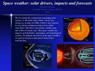
Space weather: solar drivers, impacts and forecasts Henrik Lundstedt Swedish Institute of Space Physics Lund We live inside the continuously expanding solar corona, i.e. the solar wind, which can be very strong e.g. at times of CMEs. Earth is also exposed to very intense radiation at times of so called solar flares. The Sun is also inside a stellar wind and a flow of cosmic rays. This space weather has impacts on both Earth’s atmosphere and technological systems. To mitigate the effects of the space weather we need to forecast it and start to learn to live with the Sun.
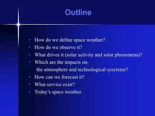
Outline • How do we define space weather? • How do we observe it? (solar weather) • What drives it? (solar activity and solar phenomena) • Which are the impacts on: the Earth’s atmosphere and technological systems? • How can we forecast it? • What services exist? • Today’s space weather.
Space weather ”Rymdväder” was mentioned the first time in media 1991! HD 1981 (cykel 21) SDS 1991 (cycle 22) Arbetet 1981 (cycle 21) SDS 1991 (cycle 22) The US National Space Weather Program 1995: ”Space weather refers to conditions on the sun, and in the solar wind, magnetosphere, ionosphere and thermosphere that can influence the performance and reliability of space-borne and ground-based technological systems and endanger human life or health”. LWS 2001 and ILWS 2002. ESA Space Weather Programme started in April 1999. ESA Space Weather Pilot projects start in April 2003. SWWT, EU COST 724 Space Weather.
Workshops arranged in Lund John Freeman (Rice University, Houston, TX) coined the word ”space weather” Workshops on ”Artificial Intelligence Applications in Solar-Terrestrial Physics” were held in Lund 1993 and 1997.
The Sun Diameter: 1 390 000 km (109 x Earth) Mass: 1.99x1030 kg (330 000 x Earth) Density: Core 151x103 kg/m-3 Average 1.41x10³ kg/m-3 The Sun consits of: H (≈ 90%) Helium (≈ 10%) C,N,O ( ≈ 0.1%) Temperature: Core 15 million Photosphere 5800 K Chromosphere 4300-104K Corona 1-30 million K 4 protons --> He + 2 positrons + 2 neutrinos + 2 fotons (26.2 MeV)
A plasma A plasma is a quasineutral gas of charged and neutral particles, which exhibits collevtive behavior. Three conditions a plasma must satisfy.
Plasma equations Macroscopic plasma quantities: By taking velocity moments of the particle distribution function fs(x,v,t) for particles of species s in six-dimensional phase space we obtain macroscopic measurable quantities such as bulk velocity, pressure and the temperature. Macroscopic equations: By taking velocity moments of the Vlasov equation we obtain the fluid equations of a plasma in terms of the macroscopic variables. The zeroth and first order moments, result in continuity equation and fluid equation of motion.
Magnetohydrodynamic (MHD) approximation Induction equation Equation of continuity Equation of motion Maxwell’ equations and Ohm’s law give the induction equation. We need to observe V and B.
Solar observations • Where on Earth do we observe the Sun? • What spacecrafts observe the Sun? • How do we observe V and B on the Sun?
Solar observations in California Big Bear Solar Observatory Mount Wilson Observatory Wilcox Solar Observatory Internet-accessible robotic solar telescope in Livermore
French solar observation facilities Pic du Midi (Coronagraph, (Lyot) THEMIS on Tenerife (solar magnetic field) Radioheliograph at Nancay (CMEs)
Solar observations with the Swedish solar telescope on La Palma
Advanced Technology Solar Telescope 4-m telescope 0.1” resolution Operational 2009 National Solar Observatory
Probing CMEs in radio wavelengths with a solar radar in Sweden 2003-2006 15 000 antennas with receivers and senders, arranged in 100 clusters distributed withi a circle of 350 kms diameter. Data transfer rate 25 Tbits/s. Frequency 10-250 MHz (30-1.5m)
ACE waslaunched in August 25, 1997 Solar wind observations with ACE make accurate forecasts 1-3 hours ahead possible.
Solar Orbiter - planned launch 2009 Study the Sun from close-up (45 solar radii, .21 au), (0.05 arcsec) latitude as high as 38 degrees
SDO - planned launch April 2008 Geosynchronous orbit
SOHO has given us a totally new picture of the Sun- always active • Solar Heliospheric Observatory was launched on December 2, 1995 • SOHO carries three instruments observing the solar interior, six the solar corona and three the solar wind
When the solar magnetic field emerges thru the solar suface sunspots appear
The Sun Diameter: 1 390 000 km (109 x Earth) Mass: 1.99x1030 kg (330 000 x Earth) Density: Core 151x103 kg/m-3 Average 1.41x10³ kg/m-3 The Sun consits of: H (≈ 90%) Helium (≈ 10%) C,N,O ( ≈ 0.1%) Temperature: Core 15 million Photosphere 5800 K Chromosphere 4300-104K Corona 1-30 million K 4 protons --> He + 2 positrons + 2 neutrinos + 2 fotons (26.2 MeV)
The oscillations reveal solar interior The oscillations at the surface of the Sun are reflections of the standing sound waves that fill the interior. Each standing wave (or n, l, m mode) is trapped between the surface and some critical depth.
A standard solar model The model must reproduce the observed luminosity and radius of the Sun at its present age from the solar mass, initial chemical composition and age. The mass equation, equation of hydrostatic equilibrium, equation for energy balance and equation for radiation energy transfer determine the evolution of the Sun. Energy transferred by radiation by convection L = luminosity (amount of energy radiated per unit time, measured in watts) e = energy generated per unit mass per unit time in the core k = opacity
When the solar magnetic field emerges thru the solar suface sunspots appear
Why sunspots live so long MDI shows how magnetic elements form sunspots (local helioseismology)
Sunspot solar cycles Schwabe found the 11- year sunspot solar cycle. R = k(10g + f). Gleissberg found the 80-90 years cycle. Maunder-Spörer 207 years cycle, Houtermans cycle 2272 years and Sharma 100 000 years cycle. The two peaks of solar activity, 1.3 years separated!
A Maunder minimum suddenly? In the beginning of 1640 the sunspot number suddenly decreased to near zero. The Maunder Minimum started 1645 and ended 1715.
Gleissberg maximum? (The Carington event 1859 September 1 produced a white light flare, >30MeV proton fluency 4-8 times ”worst case” 1972, a CME v=2500km/s, 18h later a super- storm with Dst = -1760nT!). The number of severe proton events follow the Gleissberg cycle and might increase with a factor 8-10. A maximum occurred 1980. A new warm ”Grand Maximum” (1050-1250) has been suggested by J. Lean 2030-2040.
Rapid changes for other solar type stars For a solar type star the luminosity decreased with 0.4%på in just a few years. Similar rapid changes happened during the Maunder minimum! (compare 1640-1645!) Mount Wilson studies HD 9562 (G2V) Maunder minimum state HD 136202 (F8IV) 23 years Sun (G2V) 10.0 years HD 10476 (K1V) 9.6 years HD 149661 (K0V 17.4 +4.0 years) multiple cycles HD101501 (G8V) chaotic
Non-linear chaotic solar dynamo (N. Weiss) A complex generalization of the three ordinary Lorenz diff equations. The toroidal magnetic field for a aW dynamo. As the dynamo number D increases D1 (no activity) -> D2 (cycle activity) -> D3 (chaotic activity)
aw, meridional-Dynamo Peter Gillman and Mausumi Dikpati (Astrophys. J, 2001)
Solar activity and temperatureduring longer periods J. Eddy 1976 Meton (in Greece) claimed 400 B.C. that high solar activity was related to wet climate.
Christmas day 1690 - during Maunder minimum It’s heavily snowing in Rome and on the French riviera. Children are skating on Thames River in London and they have annual frost fairs. In Amsterdam the canals are frozen. In Paris the snow is deep. Europa experienced ”Little Ice Age”.
Lund during the Middle Ages and the Maunder minimum The Danish kingdom during Knud the great (1016). During the Middle Ages Lund prospered, Lund was called the capital of Denmark (Metropolis Daniea). Rich could drink excellent wine from England (e.g. from Abbey of Abingdon). Today Bothy Vineyard, south of Oxford. The Swedish king Karl X Gustaf looks at the ice before the crossing of the Belts 1658. The battle in Lund follows in December 4, 1676 and Lund becomes Swedish.