Protein Structural Prediction
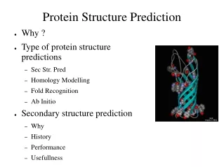
Protein Structural Prediction. Performance of Structure Prediction Methods. TRILOGY: Sequence–Structure Patterns. Identify short sequence–structure patterns 3 amino acids Find statistically significant ones (hypergeometric distribution) Correct for multiple trials


Protein Structural Prediction
E N D
Presentation Transcript
TRILOGY: Sequence–Structure Patterns • Identify short sequence–structure patterns 3 amino acids • Find statistically significant ones (hypergeometric distribution) • Correct for multiple trials • These patterns may have structural or functional importance • Pseq: R1xa-bR2xc-dR3 • Pstr: 3 C– C distances, & 3 C – C vectors • Start with short patterns of 3 amino acids {V, I, L, M}, {F, Y, W}, {D, E}, {K, R, H}, {N, Q}, {S, T}, {A, G, S} • Extend to longer patterns Bradley et al. PNAS 99:8500-8505, 2002
TRILOGY: Extension Glue together two 3-aa patterns that overlap in 2 amino acids P-score = i:Mpat,…,min(Mseq, Mstr)C(Mseq, i) C(T – Mseq, Mstr – i) C(T, Mstr)-1
TRILOGY: Longer Patterns -- unit found in three proteins with the TIM-barrel fold NAD/RAD binding motif found in several folds Type-II turn between unpaired strands Helix-hairpin-helix DNA-binding motif A -hairpin connected with a crossover to a third -strand Three strands of an anti-parallel -sheet A fold with repeated aligned -sheets Four Cysteines forming 4 S-S disulfide bonds
Small Libraries of Structural Fragments for Representing Protein Structures
protein sequence fragment library … Fragment Libraries For Structure Modeling predicted structure known structures
f Small Libraries of Protein Fragments Kolodny, Koehl, Guibas, Levitt, JMB 2002 Goal: Small “alphabet” of protein structural fragments that can be used to represent any structure • Generate fragments from known proteins • Cluster fragments to identify common structural motifs • Test library accuracy on proteins not in the initial set
f Small Libraries of Protein Fragments Dataset: 200 unique protein domains with most reliable & distinct structures from SCOP • 36,397 residues • Divide each protein domain into consecutive fragments beginning at random initial position Library: Four sets of backbone fragments • 4, 5, 6, and 7-residue long fragments • Cluster the resulting small structures into k clusters using cRMS, and applying k-means clustering with simulated annealing • Cluster with k-means • Iteratively break & join clusters with simulated annealing to optimize total variance Σ(x – μ)2
Evaluating the Quality of a Library • Test set of 145 highly reliable protein structures (Park & Levitt) • Protein structures broken into set of overlapping fragments of length f • Find for each protein fragment the most similar fragment in the library (cRMS) Local Fit: Average cRMS value over all fragments in all proteins in the test set Global Fit: Find “best” composition of structure out of overlapping fragments • Complexity is O(|Library|N) • Greedy approach extends the C best structures so far from pos’n 1 to N
Results C =
Protein Side-Chain Packing • Problem: given the backbone coordinates of a protein, predict the coordinates of the side-chain atoms • Method: decompose a protein structure into very small blocks Slide credits: Jimbo Xu
Protein Structure Prediction • Stage 1: Backbone Prediction • Ab initio folding • Homology modeling • Protein threading • Stage 2: Loop Modeling • Stage 3: Side-Chain Packing • Stage 4: Structure Refinement The picture is adapted from http://www.cs.ucdavis.edu/~koehl/ProModel/fillgap.html Slide credits: Jimbo Xu
Side-Chain Packing 0.3 0.2 0.3 0.7 0.1 0.4 0.1 0.1 0.6 clash Each residue has many possible side-chain positions Each possible position is called a rotamer Need to avoid atomic clashes Slide credits: Jimbo Xu
Energy Function Assume rotamer A(i) is assigned to residue i. The side-chain packing quality is measured by clash penalty 10 clash penalty 0.82 1 occurring preference The higher the occurring probability, the smaller the value : distance between two atoms :atom radii Minimize the energy function to obtain the best side-chain packing. Slide credits: Jimbo Xu
Related Work • NP-hard [Akutsu, 1997; Pierce et al., 2002] and NP-complete to achieve an approximation ratio O(N) [Chazelle et al, 2004] • Dead-End Elimination: eliminate rotamers one-by-one • SCWRL: biconnected decomposition of a protein structure [Dunbrack et al., 2003] • One of the most popular side-chain packing programs • Linear integer programming [Althaus et al, 2000; Eriksson et al, 2001; Kingsford et al, 2004] • Semidefinite programming [Chazelle et al, 2004] Slide credits: Jimbo Xu
Algorithm Overview • Model the potential atomic clash relationship using a residue interaction graph • Decompose a residue interaction graph into many small subgraphs • Do side-chain packing to each subgraph almost independently Slide credits: Jimbo Xu
Residue Interaction Graph • Vertices: Each residue is a vertex • Edges: Two residues interact if there is a potential clash between their rotamer atoms h f b d s m c a e i j k l Residue Interaction Graph Slide credits: Jimbo Xu
Key Observations • A residue interaction graph is a geometric neighborhood graph • Each rotamer is bound to its backbone position by a constant distance • No interaction edge between two residues if distance > D • D: constant depending on rotamer diameter • A residue interaction graph is sparse! Slide credits: Jimbo Xu
Tree Decomposition[Robertson & Seymour, 1986] • Definition. A tree decomposition (T, X) of a graph G = (V, E): • T=(I, F) is a tree with node set I and edge set F • X is a set of subsets of V, the components; Union of elts. in X = V • 1-to-1 mapping between I and X • For any edge (v,w) in E, there is at least one X(i) in X s.t. v, w are in X(i) • In tree T, if node j is on the path from i to k, then X(i) ∩ X(k) X(j) • Tree width is defined to be the maximal component size minus 1 Slide credits: Jimbo Xu
h f d f abd b d g g m c m c a e i a e i j l k j k l Tree Decomposition[Robertson & Seymour, 1986] Greedy: minimum degree heuristic h • Choose the vertex with minimal degree • The chosen vertex and its neighbors form a component • Add one edge to any two neighbors of the chosen vertex • Remove the chosen vertex • Repeat the above steps until the graph is empty Slide credits: Jimbo Xu
h fgh f b d g m acd cdem defm abd c a e i clk eij j k l Tree Decomposition (Cont’d) Tree Decomposition Tree width: size of maximal component – 1 Slide credits: Jimbo Xu
Side-Chain Packing Algorithm Xr Xir Bottom-to-Top: Calculate the minimal energy function Top-to-Bottom: Extract the optimal assignment Time complexity: Exponential in tree width, linear in graph size Xi Xp Xq Xj Xl Xli Xji A tree decomposition rooted at Xr Score of component Xi Score of subtree rooted at Xl Score of subtree rooted at Xi Score of subtree rooted at Xj Slide credits: Jimbo Xu
Empirical Component Size Distribution Tested on the 180 proteins used by SCWRL 3.0. Components with size ≤ 2 ignored. Slide credits: Jimbo Xu
Result Theoretical time complexity: << is the average number rotamers for each residue. Five times faster on average, tested on 180 proteins used by SCWRL Same prediction accuracy as SCWRL 3.0 CPU time (seconds) Slide credits: Jimbo Xu
Accuracy A prediction is judged correct if its deviation from the experimental value is within 40 degree. Slide credits: Jimbo Xu