Download

1 / 75
750 likes | 915 Views
Econ 2019 - Matrix Algebra UNIT 3 Determinants. Fall 2010 Christine Clarke, PhD UWI Mona. Recap. Row and Reduced Row Echelon Elementary Matrices. Gaussian Elimination and Gauss-Jordan Elimination.

E N D
Econ 2019 - Matrix AlgebraUNIT 3 Determinants Fall 2010 Christine Clarke, PhD UWI Mona
Recap Row and Reduced Row Echelon Elementary Matrices
If m and n are positive integers, then an m n matrixis a rectangular array in which each entryaij of the matrix is a number. The matrix has m rows and n columns.
Terminology A real matrix is a matrix all of whose entries are real numbers. i (j) is called the row (column) subscript. An mn matrix is said to be of size (or dimension) mn. If m=n the matrix is square of order n. The ai,i’s are the diagonal entries.
Given a system of equations we can talk about its coefficient matrix and its augmented matrix. These are really just shorthand ways of expressing the information in the system. To solve the system we can now use row operations instead of equation operations to put the augmented matrix in row echelon form.
Elementary Row Operations 1. Interchange two rows. 2. Multiply a row by a nonzero constant. 3. Add a multiple of a row to another row.
Two matrices are said to be row equivalent if one can be obtained from the other using elementary row operations. • A matrix is in row-echelon form if: • All rows consisting entirely of zeros are at the bottom. • In each row that is not all zeros the first entry is a 1. • In two successive nonzero rows, the leading 1 in the higher row is further left than the leading 1 in the lower row.
Gaussian Elimination with Matrices 1. Write the augmented matrix of the system. 2. Use elementary row operations to find a row equivalent matrix in row-echelon form. 3. Write the system of equations corresponding to the matrix in row-echelon form. 4. Use back-substitution to find the solutions to this system.
Gauss Jordan Elimination In Gauss-Jordan elimination, we continue the reduction of the augmented matrix until we get a row equivalent matrix in reduced row-echelon form. (r-e form where every column with a leading 1 has rest zeros)
Homogeneous Systems A system of linear equations in which all of the constant terms is zero is called homogeneous. All homogeneous systems have the solutions where all variables are set to zero. This is called the trivial solution.
New Stuff Using Elementary Matrices
Elementary Matrices An n by n matrix is called an elementary matrix if it can be obtained from Inby a single elementary row operation. These matrices allow us to do row operations with matrix multiplication.
Representing Elementary Row Operations Theorem: Let E be the elementary matrix obtained by performing an elementary row operation on In. If that same row operation is performed on an m by n matrix A, then the resulting matrix is given by the product EA.
Three types of Elementary Matrices These correspond to the three types of EROs that we can do: Interchanging rows of I -> Type I EM Multiplying a row of I by a constant -> Type II EM Adding a multiple of one row to another -> Type III EM
Type I EM E1 = How is this created? Eg. 1 Suppose A = E1A = = What is AE1?
Type II EM E2 = E2A = = AE2 = =
Type III EM E3 = E3A = = AE3 = =
Row equivalent matrices Let A and B be m by n matrices. Matrix B is row equivalent to A if there exists a finite number of elementary matrices E1, E2, ... Eksuch that B = EkEk-1 . . . E2E1A.
Break it down This means that B is row equivalent to A if B can be obtained from A through a series of finite row operations. If we then take two augmented matrices (A|b) and (B|c) and they are row equivalent, then Ax = b and Bx=c must be equivalent series
Break it down If A is row equivalent to B, B is row equivalent to A If A is row equivalent to B and B is row equivalent to C then A is row equivalent to C
Example Compute the inverse of A for A =
Example Now, solve the system:
Example We can employ the format Ax = b so x=A-1b We just calculated A-1 and b is the column vector So we can easily find the values of x by multiplying the two matrices
Determinants Keys to calculating Inverses
Determinants • Require square matrices • Each square matrix has a determinant written as det(A) or |A| • Determinants will be used to: • characterize on-singular matrices • express solutions to non-singular systems • calculate dimension of subspaces
Properties of Determinants If A and B are square then It is not difficult to appreciate that If A has a row (or column) of zeros then If A has two identical rows (or columns) then
Properties of Determinants If B is obtained from A by ERO, interchanging two rows (or columns) then If B is obtained from A by ERO where row (or column) of A were multiplied by a scalar k, then
Properties of Determinants If B is obtained from A by ERO where a multiple of a row (or column) of A were added to another row (or column) of A then
For a 2 by 2 matrix That Is the determinant is equal to the product of the elements along the diagonal minus the product of the elements along the off-diagonal.
Example Note: The matrix A is said to be invertible or non-singular if det(A)≠ 0. If det(A) = 0, then A is singular.
For a 3 by 3 matrix Using EROs on rows 2 and 3
For a 3 by 3 matrix The matrix will be row equivalent to I iff:
For a 3 by 3 matrix This implies that the Det(A) =
Using EROs to find the Det. • Use EROs to find:
Using EROs to find the Det. • STEP 1: Apply from property 5 this gives us • STEP 2: Convert matrix to Echelon form
Using EROs to find the Det. • Therefore is the same as: matrix is now in echelon form so we can multiply elements of main diagonal to get determinant
Example • Factorize the determinants of • What is ?
Example cont’d • We see that y – x is a factor of row 2 and z – x is a factor of row 3 so we factor them out from: • And we get:
Example cont’d • The matrix is now in echelon form so we can multiply elements of main diagonal to get determinant and then multiply by factors to get: =
Example cont’d • Now, the matrix corresponds to • Since =
Example cont’d • Then =
Now for n by n’s • Cofactor expansion is one method used to find the determinant of matrices of order higher than 2.
Minor of a Matrix • If A is a square matrix, then the minorMi,jof the element ai,jof A is the determinant of the matrix obtained by deleting the ith row and the jth column from A.
Example • Consider the matrix . The minor of the entry “0” is found by deleting the row and the column associated with the entry “0”.
Example cont’d • The minor of the entry “0” is Note: Since the 3 x 3 matrix A has 9 elements there would be 9 minors associated with the matrix.
Cofactor of a Matrix • The cofactorCi,j= (-1)i+jMi,j. Since we can think of the cofactor of as nothing more than its signed minor.
Example • Find the minor and cofactor of the entry “2” for • We first need to delete the row and column corresponding to the entry “2”
Example cont’d • The Minor of 2 is • The minor corresponds to row 1 and column 2 so applying the formula, we have • So the cofactor of the entry “2” is 40.