Download
1 / 81
810 likes | 1k Views
operating systems. Scheduling. operating systems. There are a number of issues that affect the way work is scheduled on the cpu. operating systems. Batch vs. Interactive. operating systems. Batch System vs. Interactive System. Scheduling Issues.

E N D
operating systems Scheduling
operating systems There are a number of issues that affect the way work is scheduled on the cpu.
operating systems Batch vs. Interactive
operating systems Batch System vs. Interactive System Scheduling Issues In a batch system, there are no users impatiently waiting at terminals for a quick response. On large mainframe systems where batch jobs usually run, CPU time is still a precious resource. Metrics for a batch system include * Throughput – number of jobs per hour that can be run * Turnaround – the average time for a job to complete * CPU utilization – keep the cpu busy all of the time
operating systems Batch System vs. Interactive System Scheduling Issues In interactive systems the goal is to minimize response times. Proportionality – complex things should take more time than simple things. Closing a window should be immediate. Making a dial-up connection would be expected to take a longer time. One or two users should not be able to hog the cpu
operating systems Single vs Multiple User
operating systems Single User vs. Multi-User Systems Scheduling is far less complex on a single user system: * In today’s Personal computers (single user systems), it is rare for a user to run multiple processes at the same time. * On a personal computer most wait time is for user input. * CPU cycles on a personal computer are cheap. Scheduling Issues
operating systems Compute vs. I/O Bound Programs Most programs exhibit a common behavior, they compute for a while, Then they do some I/O. Scheduling Issues Compute Bound: Relatively long bursts of CPU activity with short intervals waiting for I/O I/O Bound: Relatively short bursts of CPU activity with frequent long waits for I/O
operating systems When to Schedule Job Scheduling: When new jobs enter the system Select jobs from a queue of incoming jobs and place them on a process queue where they will be subject to Process Scheduling. The goal of the job scheduler is to put jobs in a sequence that will use all of the system’s resources as fully as possible. Scheduling Issues Example: What happens if several I/O bound jobs are scheduled at the same time?
operating systems When to Schedule Scheduling Issues Process Scheduling or Short Term Scheduling: For all jobs on the process queue, Process Scheduling determines which job gets the CPU next, and for how long. It decides when processing should be interrupted, and when a process completes or should be terminated.
operating systems Scheduling Issues Preemptive vs. non-Preemptive Scheduling Non-preemptive scheduling starts a process running and lets it run until it either blocks, or voluntarily gives up the CPU. Preemptive scheduling starts a process and only lets it run for a maximum of some fixed amount of time.
operating systems Pick the criteria that are important to you. One algorithm cannot maximize all criteria. Scheduling Criteria Turnaround time – complete programs quickly Response Time – quickly respond to interactive requests Deadlines – meet deadlines Predictability – simple jobs should run quickly, complex job longer Throughput – run as many jobs as possible over a time period
operating systems continued Scheduling Criteria CPU Utilization – maximize how the cpu is used Fairness – give everyone an equal share of the cpu Enforcing Priorities – give cpu time based on priority Enforcing Installation Policies – give cpu time based on policy Balancing Resources – maximize use of files, printers, etc
Pre-emption or voluntary yield Ready List CPU Scheduler new PCB PCB running PCB ready request Resource Mgr allocate PCB PCB resources blocked
A process entering ready state Ready List Scheduler PCB Enqueuer To the CPU Dispatcher Context Switcher
The cost of a context switch Assume that your machine has 32-bit registers The context switch uses normal load and store ops. Lets assume that it takes 50 nanoseconds to store the contents of a register in memory. If our machine has 32 general purpose registers and 8 status registers, it takes (32 + 8 ) * 50 nanoseconds = 2 microseconds to store all of the registers.
Another 2 microseconds are required to load the registers for the new process. Keep in mind that the dispatcher itself is a process that requires a context switch. So we could estimate the total time required to do a context switch as 8+ microseconds. On a 1Gh machine, register operations take about 2 nanoseconds. If we divide our 8 microseconds by 2 nanoseconds we could execute upwards of 4000 register instructions while a context switch is going on. This only accounts for saving and restoring registers. It does not account for any time required to load memory.
Given a set of processes where the cpu time required for each to complete is known beforehand, it is possible to select the best possible scheduling of the jobs, if - we assume that no other jobs will enter the system - we have a pre-emptive scheduler - we have a specific goal (i.e. throughput) to meet Optimal Scheduling This is done by considering every possible ordering of time slices for each process, and picking the “best” one. But this is not very realistic – why not?
Given a set of processes where the cpu time required for each to complete is known beforehand, it is possible to select the best possible scheduling of the jobs, if - we assume that no other jobs will enter the system - we have a pre-emptive scheduler - we have a specific goal (i.e. throughput) to meet Optimal Scheduling This is done by considering every possible ordering of time slices for each process, and picking the “best” one. This could take more time than actually running the thread! But this is not very realistic – why not? Are there any examples where these requirements hold?
P = {pi | 0 < i < n} Scheduling Model P is a set of processes Each process pi in the set is represented by a descriptor {pi, j} that specifies a list of threads. Each thread contains a state field S(pi, j) such that S(pi, j) is one of {running, blocked, ready}
Some Common Performance Metrics Service Time(pi,j) The amount of time a thread needs to be in running state until it is completed. Wait TimeW (pi,j) The time the thread spends waiting in the ready state before its first transition to running state. * Turnaround TimeT (Pi, j) The amount of time between the moment the thread first enters the ready state and the moment the thread exits the running state for the last time. * Silberschatz uses a different definition of wait time.
Some Common Performance Metrics Response TimeT (Pi, j) In an interactive system, one of the most important performance metrics is response time. This is the time that it takes for the system to respond to some user action.
System Load If is the mean arrival rate of new jobs into the system, and is the mean service time, then the fraction of the time that the cpu is busy can be calculated as p = / . This assumes no time for context switching and that the cpu has sufficient capacity to service the load. Note: This is not the same lambda (λ) we saw a few slides back.
For example, given an average arrival rate of 10 threads per minute and an average service time of 3 seconds, = 10 threads per minute = 20 threads per minute ( 60 / 3) p = 10 / 20 = 50% What can you say about this system if the arrival rate, , is greater than the mean service time, ?
Scheduling Algorithms First-Come First Served Shortest Job First Priority Scheduling Deadline Scheduling Shortest Remaining Time Next Round Robin Multi-level Queue Multi-level Feedback Queue
The simplest of scheduling algorithms. The Ready List is a fifo queue. When a process enters the ready queue, it’s PCB is linked to the tail of the queue. When the CPU is free, the scheduler picks the process that is at the head of the queue. First-come first-served is a non-preemptive scheduling algorithm. Once a process gets the CPU it keeps it until it either finishes, blocks for I/O, or voluntarily gives up the CPU. First-Come First-Served
When a process blocks, the next process in the queue is run. When the blocked process becomes ready, it is added back in to the end of the ready list, just as if it were a new process.
Waiting times in a First-Come First-Served System can vary substantially and can be very long. Consider three jobs with the following service times (no blocking): i i 1 24ms 2 3ms 3 3ms If the processes arrive in the order p1, p2, and then p3 P1 P2 P3 Gannt Chart 0 24 27 30 Compute each thread’s turnaround time T (p1) = (p1) = 24ms T (p2) = (p2) + T (P1) = 3ms + 24ms = 27ms T (p3) = (p3) + T (p2) = 3ms + 27ms = 30ms Average turnaround time = (24 + 27 + 30)/3 = 81 / 3 = 27ms
Waiting times in a First-Come First-Served System can vary substantially and can be very long. Consider three jobs with the following run times (no blocking): i i 1 24ms 2 3ms 3 3ms If the processes arrive in the order p1, p2, and then p3 P1 P2 P3 0 24 27 30 Compute each thread’s wait time W (p1) = 0 W (p2) = T (P1) = 24ms W (p3) = T (p2) = 27ms Average wait time = (0 + 24 + 27 ) / 3 = 51 / 3 = 17ms
Note how re-ordering the arrival times can significantly alter the average turnaround time and average wait time! i i 1 3ms 2 3ms 3 24ms P2 P3 P1 0 3 6 30 Compute each thread’s turnaround time T (p1) = (p1) = 3ms T (p2) = (p2) + T (P2) = 3ms + 3ms = 6ms T (p3) = (p3) + T (p2) = 6ms + 24ms = 30ms Average turnaround time = (3 + 6 + 30)/3 = 39 / 3 = 13ms
Note how re-ordering the arrival times can significantly alter The average turnaround and average wait times. i i 1 3ms 2 3ms 3 24ms P2 P3 P1 0 3 6 30 Compute each thread’s wait time W (p1) = 0 W (p2) = T (P1) = 3ms W (p3) = T (p2) = 6ms Average wait time = (0 + 3 + 6 ) / 3 = 9 / 3 = 3ms
Try your hand at calculating average turnaround and average wait times. i i 1 350ms 2 125ms 3 475ms 4 250ms 5 75ms
i i 1 350ms 2 125ms 3 475ms 4 250ms 5 75ms 100 400 500 600 700 800 900 1000 1100 200 300 1200
Try your hand at calculating average turnaround and average wait times. i i 1 350ms 2 125ms 3 475ms 4 250ms 5 75ms p4 p5 p1 p2 p3 1275 475 1200 0 350 950 Average turnaround = (350 + 475 + 950 + 1200 + 1275) / 5 = 850 Average wait time = (0 + 350 + 475 + 950 + 1200) / 5 = 595
The Convoy Effect Assume a situation where there is one CPU bound process and many I/O bound processes. What effect does this have on the utilization of system resources?
The Convoy Effect Blocked CPU I/O Ready Queue I/O CPU I/O
I/O I/O I/O The Convoy Effect Blocked CPU Ready Queue
I/O CPU I/O I/O The Convoy Effect Blocked CPU Ready Queue
I/O CPU I/O I/O The Convoy Effect Blocked CPU Run a long time Ready Queue Remember, first come first served scheduling is non-preemptive.
Shortest Job Next scheduling is also a non-preemptive algorithm. The scheduler picks the job from the ready list that has the shortest expected CPU time. It can be shown that the Shortest Job Next algorithm gives the shortest average waiting time. However, there is a danger. What is it? Shortest Job Next Scheduling starvation for longer processes as long as there is a supply of short jobs.
Consider the case where the following jobs are in the ready list: Process i 1 6ms 2 8ms 3 7ms 4 3ms Scheduling according to predicted processor time: P4 P1 P3 P2 0 3 9 16 24 Average turnaround time = (3 + 9 + 16 +24)/4 = 13ms
Consider the case where the following jobs are in the ready list: Process i 1 6ms 2 8ms 3 7ms 4 3ms Scheduling according to predicted processor time: P4 P1 P3 P2 0 3 9 16 24 Average wait time = (0 + 3 + 9 +16)/4 = 7ms If we were using fcfs scheduling the average wait time would have been 10.25ms.
There is a practical issue involved in actually implementing SJN, can you guess what it is? You don’t know how long the job will really take!
For batch jobs the user can estimate how long the process will take and provide this as part of the job parameters. Users are motivated to be as accurate as possible, because if a job exceeds the estimate, it could be kicked out of the system. In a production environment, the same jobs are run over and over again (for example, a payroll program), so you could easily base the estimate on previous runs of the same program.
n ∑ 1 n Sn+1 = Ti i=1 For interactive systems, it is possible to predict the time for the next CPU burst of a process based on its history. Consider the following: Where Ti = processor execution time for the ith burst Si = predicted time for the ith instance
n ∑ 1 n Sn+1 = Ti 1 n n – 1 n Sn+1 = T + S i=1 n n To avoid recalculating the average each time, we can write this as It is common to weight more recent instances more than earlier ones, Because they are better predictors of future behavior. This is done with a technique called exponential averaging. Sn+1 = Tn - (1 - )Sn
In priority scheduling, each job has a given priority, and the Scheduler always picks the job with the highest priority to run next. If two jobs have equal priority, they are run in FCFS order. Priorities range across some fixed set of values. It is up to the scheduler to define whether or not the lowest value is also the lowest priority. Note that shortest job next scheduling is really a case of priority scheduling, where the priority is the inverse of the predicted time of the next cpu burst. Priority scheduling can either be preemptive or not. Priority Scheduling
Priorities can be assigned internally or externally. Internally assigned priorities are based on various characteristics of the process, such as * memory required * number of open files * average cpu burst time * i/o bound or cpu bound Externally assigned priorities are based on things such as * the importance of the job * the funds being used to pay for the job * the department that owns the job * other, often political, factors
Real-time systems are characterized by having threads that must complete execution prior to some time deadline. The critical performance measurement of such a system is whether the system will be able to meet the scheduling deadlines for all such threads. Measures of turnaround time and wait time are irrelevant. Deadline Scheduling