Download
1 / 49
630 likes | 944 Views
Simulation of Communication Systems. Professor Z. Ghassemlooy Optical Communications Research Group http://soe.unn.ac.uk/ocr/ School of Computing, Engineering and Information Sciences University of Northumbria at Newcastle, UK. Eng. of S/W Pro., India 2009. Outline of Presentation.

E N D
Simulation of Communication Systems Professor Z. Ghassemlooy Optical Communications Research Group http://soe.unn.ac.uk/ocr/ School of Computing, Engineering and Information Sciences University of Northumbria at Newcastle, UK Eng. of S/W Pro., India 2009
Outline of Presentation • Communications Systems • Simulation software types • Case Studies based on Matlab • Concluding Remarks
Telecommunications Research Areas Eng. of S/W Pro., India 2009
Photonics - Applications • Photonics in communications: expanding and scaling Metropolitan Home access Long-Haul Board -> Inter-Chip -> Intra-Chip • Photonics: diffusing into other application sectors Health(“bio-photonics”) Environment sensing Security imaging
Wireless Wired Indoor Free-Space Optics (FSO) School of Computing, Engineering and Information Sciences – Research Optical Communications Optical Fibre Communications Photonic Switching • Pulse Modulations • Equalisation • Error control coding • Artificial neural network & • Wavelet based receivers • Fast switches • All optical routers • Chromatic dispersion • compensation using • optical signal processing • Pulse Modulations • Optical buffers • Optical CDMA • Subcarrier modulation • Spatial diversity • Artificial neural network/Wavelet based receivers 6 Eng. of S/W Pro., India 2009
OCRG – People • Staff • Prof. Z Ghassemlooy • J Allen • Dr R Binns • Dr K Busawon • Dr W. P. Ng • Visiting Academics • Prof. V Ahmadi, Univ. Of TarbiateModaress , Tehran, Iran • Dr M. H. Aly, 2Arab Academy for Scie. and Tech. and Maritime Transport, Egypt • Prof. J.P. Barbot, France • Prof. I. Darwazeh, Univ. College London • Prof. H. Döring, HochschuleMittweida Univ. of Applied Scie. (Germany) • Prof. E. Leitgeb, Graz Univ. of Techn. (Austria) • PhD Students • M. Amiri, A. Chaman-Motlagh, M. F. Chiang, M. A. Jarajreh, R. Kharel, S. Y Lebbe, W. • Loedhammacakra, Q. Lu, V. Nwanafio, E. K. Ogah, W. O. Popoola, S. Rajbhandari, A. • Shalaby, X. Tang • MSc and Beng: A Burton, D Bell, G Aggarwal, M Ljaz, O Anozie, W Leong , S Satkunam 7 Eng. of S/W Pro., India 2009
Simulation –Introduction • In recent years there has been a rapid growth in application of computer simulation in communication engineering. • Hardware becoming more complex and costly • A way forward to many researcher and teachers is to implements ideas in the software environment. • This allows testing of the system using idealised processing elements, which may take a significant time to design and realise in hardware.
Simulation –Introduction • Can support the hardware design by giving optimised component values, for the critical parts, and an early indication of the performance of the system • Allowing users to study or try things that would be difficult or impossible in real life • Simulations are particularly useful when a real-life process: • is too dangerous, • takes too long, • is too quick to study, • is too expensive to create.
Simulation Tools - Some Features • Reliability - Depend on the validity of the simulation model, therefore verification and validation are very important • Reproducibility of results • User friendly, simple and flexible (allowing user defined functions) • Extensive details of theory adopted • High speed, precession and accuracy • Hidden source code + Up to date library • Debugging capabilities and Scalability • Can readily be upgraded and updated • Cost effective and time saving
Simulation Tools - Disadvantages • Poor modelling or poor data collection can lead to: • inaccuracy or • completely misleading results • Obsession - can lead to superficial understanding and no experimental verification • However, simulation tools have become integral part of today’s research and teaching activities • Mainly for cost reasons
Simulation Software –Application in Engineering Eng. of S/W Pro., India 2009
Simulation Software –Key Features • Numerical Integration procedures • E.g. Matlab has a number of procedures • Rung-Kutta 45 – Most advanced and ideal for analogue systems • Rung-Kutta 45 • Stiff Adam with a fixed step integration – Used for discrete systems • Euler – The most basic and used for slow varying discrete systems • Ability to plot and display graphs • 2D, 3D visualisation • Simplicity for programming • Compatibility with other software
Simulation Tools –Types • Matlab/Simulink • Orcad/Pspice • VPI • Mathcad • OptSim ™ 4.0: simulation and design of advanced fiber optic communication systems • OptiSystem: large scale system software • OptiFDTD
Matlab/Simulink • A high-performance language for technical computing • Integrates computation, visualization, and programming in an easy-to-use environment • Typical uses include: • Math and computation • Algorithm development • Data acquisition • Modelling, simulation, and prototyping • Data analysis, exploration, and visualization • Scientific and engineering graphics • Application development, including graphical user interface building • Compatible with excel, uses Maple and is compatible with other software packages such as C, C++, VPI, etc.
Orcad/Pspice • To model circuits with mixed analogue and digital devices • Software-based circuit breadboard for test and refinement • Can perform: • AC, DC, and transient analyses • Parametric, Monte Carlo, and sensitivity/worst-case analyses – i.e. circuit behaviour in a changing environment • Digital worst-case timing analysis : to resolve timing problems occurring with only certain combinations of slow and fast signal transmissions, etc. • Not compatible with excel
Mathcad • A desktop software for performing and documenting engineering and scientific calculations • Equations and expressions are displayed graphically (WYSIWYG) • Capabilities : • Solving differential equations - several possible numerical methods • Graphing functions in two or three dimensions • Symbolic calculations including solving systems of equations • Vector and matrix operations including eigenvalues and eigenvectors • Curve fitting • Finding roots of polynomials and functions • Statistical functions and probability distributions • Calculations in which units are bound to quantities • One can’t use symbolic parameters only numerical parameters
OptiSystem • Is used for • designing, testing and optimization of virtually any type of optical links in the physical layers • based on a large collection of realistic models for components and sub-systems • OptiFDTD (finite-difference time-domain) • propagation of optical fields through nano- to micro-scaled devices by directly solving Maxwell’s equations numerically
OptiSystem – contd. • OptiBPM • Based on the beam propagation method (BPM) • a semi-analytical technique that solves an approximation of the wave equation • Waveguide other similar optical devices • Light propagation predominantly in one direction over large distances
Virtual Photonics Inc. • Used in optical networks and optical devices modelling • Support C and Matlab • Will talk about this in my second lecturer!
Channel code word Message signal Modulated Transmitted signal Source Encoder Channel Encoder Mod- ulator Source Source Decoder Channel Decoder Demod- ulator User Received signal Estimate of message signal Estimate of channel code word Case Studies - MATLAB A typical communication system block diagram Channel
Case Study 1 - AM/FM communication system s • Aim: To simulate a communication system link Tasks: • Channel modeling • Comparing received and transmitted signals • System performance evaluation • System optimization • Final system design
AM/FM Simulation - System Parameters Know parameters • Carrier frequency, and power • Signal bandwidth • Modulation index • Channel bandwidth and loss • Link length • Transmitter/receiver antenna type and gain Performance parameters • Output signal-to-noise vs carrier to noise ratio • System linearity • Harmonic distortions
FM – Simulation Block Diagram Message FM modulator Amplifier Transmitter Channel Amplifier Receiver Low pass filter FM demodulator Recovered Message
FM Simulation - Matlab-Simulink • Provided that the mathematics underlying each block is fully appreciated, one could use any programming languages including high level computer languages C, C++, Java or scientific programming languages Matlab, MathCAD , Mathematica, Octave to name a few • Matlab/Simulink • One of the most popular simulation tool available • Simulink is more user friendly for beginners as there are many drag and drop block functions. • However Simulink also sometimes limits flexibility to users.
FM Simulation - Performance Evaluation • The easiest way to evaluate the performance is by visual inspections • For example, one can hardly differentiate between the transited message and recover message in the previous example • Message signal at different SNRs is shown below- observe the improvement in the performance with increasing SNRs
FM Simulation - Performance Evaluation • Visual inspection is the simplest and in many cases gives an insight to the system, BUT it is very error prone • Alternative method of analysis should be used • Considered error signal defined as: error = (m - mr)2 • The error signal at SNRs of 15, 20 and 40 is shown below • The performance difference between the SNRs of 15 and 20 is apparent
FM Simulation - Performance Evaluation • Simulation software may provide many interesting results, but the expertise and experience of the user play's a major role • In previous plot - very little difference between 20 dB and 40 dB • An experienced user may choose the log-scale to plot error to gain more information, shown below • Compared to the pervious plot, difference in performance for 20 db and 40 dB is clear from this plot
Case study 2- Digital Communications • Depending upon the channel, receiver may incorporated other signal processing tools like equalizing filter, low pass filter and so on • The output bits are compared to the transmitted to bit to calculated the error • The bit error rate (BER) is the metric used in all digital communication system to compare and evaluate the system performance • BER depends on the SNR (valid only for particular signalling format):
Modelling Approach • A discrete model based on mathematical analysis is generated and model using the simulation software • Discrete-time equivalent system of digital communication system is defined as: ri = Eb+ni if bi=1 ri = ni if bi=0 ri is the sampled output Ebis the energy per bit and ni is the additive white Gaussian noise • Performance evaluation: • bit error rate • eye-diagram
Digital Simulation - Performance Evaluation • BER of different modulation techniques for indoor optical wireless system
Digital Simulation - Notes • To properly model the system, it is necessary to understand mathematics involved in each and every module • Code are written to approximate the mathematical equations. The code are grouped together and put as a block for simple user interface • Example: Matlab codes for noise signal:
Digital Simulation – Matlab Codes Fixed and variable parameters clear clc close all fs = 6.0e+6; %sampling frequency 6 MHz ts = 1/fs; %Sampling time fc = ; %clock signal frequency ac:; %clock signal peak amplitude n = 2*(6*fs/fc); %Maximum number of points w.r.t the 6 cycles of clock signal fc nc = 6; %Number cycls of clock signal to be shown tmax= nc*tc; %Maximum number of point in 6 cycles of fc fmax = (2*n*fc/fs); %Maximum frequency range final = ts*(n-1); % maximum time t = 0:ts:tmax; %time vector for sketching waveform in time domain
Digital Simulation – Matlab Codes Data signal generated from the Clock Signal L length (sq); %All the values of clock signal is assigned to a new variable l da = sq; %Set initial values out=1; temp=1; for i=1:L-1 if sq(i)== -2.5 & sq(i+1)== 2.5 %Reverse output voltage polarity temp= out * -1; out=temp; end %Change value of out to +/-1 if out>0 out=1; else out= -1; end da(i)=out; %data signal at half the clock frequency end %Set value of final element of da da(L)=out; %Plot data signal
Optical Wireless Communication What does It Offer ? Abundance of unregulated bandwidth - 200 THz in the 700-1500 nm range No multipath fading - Intensity modulation and direct detection High data rate – In particular line of sight (in and out doors) Improved wavelength reuse capability Flexibility in installation Secure transmission Flexibility - Deployment in a wide variety of network architectures. Installation on roof to roof, window to window, window to roof or wall to wall.
Access Network Bottleneck (Source: NTT) Eng. of S/W Pro., India 2009
POINT B Free Space Optics • Cloud • Rain • Smoke • Gases • Temperature variations • Fog and aerosol DRIVER CIRCUIT SIGNAL PROCESSING The transmission of optical radiation through the atmosphere obeys the Beer-Lamberts’s law: Preceive = Ptransmit * exp(-αL) PHOTO DETECTOR α : Attenuation coefficient POINT A This equation fundamentally ties FSO to the atmospheric weather conditions Link Range L 39 Eng. of S/W Pro., India 2009
. . . . Case Study 3: Optical Wireless Systems DC bias m(t) m(t)+bo d(t) Summing circuit Optical transmitter Subcarrier modulator Serial/parallel converter Data in Atmospheric channel ir d’(t) Subcarrier demodulator Spatial diversity combiner Photo- detector array Parallel/serial converter . . Data out 40 Eng. of S/W Pro., India 2009
Subcarrier Modulation - Transmitter Eng. of S/W Pro., India 2009
Photo-current R = Responsivity, I = Average power, = Modulation index, m(t) = Subcarrier signal Subcarrier Modulation - Receiver 42 Eng. of S/W Pro., India 2009
Error Performance – Bit Error Performance BPSK BER against SNR for M-ary-PSK for log intensity variance = 0.52 BPSK based subcarrier modulation is the most power efficient Eng. of S/W Pro., India 2009 43
TX Data in Channel + Noise Slicer Data out … MMSE MF Slicer Equaliser Data out CWT Slicer NN Data out Wavelet - NN Receiver Models Eng. of S/W Pro., India 2009
Wavelet-AI Receiver - Advantages and Disadvantages • Complexity - many parameters & computation power • High sampling rates - technology limited • Speed - long simulation times on average machines • Similar performance to other techniques • Data rate independent - data rate changes do not affect structure (just re-train) • Relatively easy to implement with other pulse modulation techniques
Wavelet Wavelet-AI Receiver SNR Vs. the RMS delay spread/bit duration
Final Remarks • Simulation software provide scientist and engineers with additional tools to implement, assess and modify ideas with a press of a button • Detailed mathematical understanding is essential • High speed and parallel processing is the way forward • Should never be a substitute to real practical systems
Thank you for your attention ! Any questions?
Acknowledgements • To R Kharel, S Rajbhandari, W Popoola, and other PhD students, • Northumbria University and CEIS School for Research Grants Z Ghassemlooy