Multiple Comparison Procedures
Multiple Comparison Procedures.

Multiple Comparison Procedures
E N D
Presentation Transcript
Multiple Comparison Procedures Once we reject H0: ==...c in favor of H1: NOT all ’s are equal, we don’t yet know the way in which they’re not all equal, but simply that they’re not all the same. If there are 4 columns, are all 4 ’s different? Are 3 the same and one different? If so, which one? etc.
These “more detailed” inquiries into the process are called MULTIPLE COMPARISON PROCEDURES. Errors (Type I): We set up “” as the significance level for a hypothesis test. Suppose we test 3 independent hypotheses, each at = .05; each test has type I error (rej H0 when it’s true) of .05. However, P(at least one type I error in the 3 tests) = 1-P( accept all ) = 1 - (.95)3 .14 3, given true
In other words, Probability is .14 that at least one type one error is made. For 5 tests, prob = .23. Question - Should we choose = .05, and suffer (for 5 tests) a .23 OVERALL Error rate (or “a” or aexperimentwise)? OR Should we choose/control the overall error rate, “a”, to be .05, and find the individual test by 1 - (1-)5 = .05, (which gives us = .011)?
The formula 1 - (1-)5 = .05 would be valid only if the tests are independent; often they’re not. [ e.g., 1=22=3, 1= 3 IF accepted & rejected, isn’t it more likely that rejected? ] 2 3 1 1 2 3
When the tests are not independent, it’s usually very difficult to arrive at the correct for an individual test so that a specified value results for the overall error rate.
Categories of multiple comparison tests - “Planned”/ “a priori” comparisons (stated in advance, usually a linear combination of the column means equal to zero.) - “Pairwise” comparisons (every column mean compared with each other column mean) - “Post hoc”/ “a posteriori” comparisons (decided after a look at the data - which comparisons “look interesting”)
(Pairwise comparisons are traditionally considered as “post hoc” and not “a priori”, if one needs to categorize all comparisons into one of the two groups) There are many multiple comparison procedures. We’ll cover only a few. Method 1: Do a series of pairwise t-tests, each with specified value (for individual test). This is called “Fisher’s LEAST SIGNIFICANT DIFFERENCE” (LSD).
Example: Broker Study A financial firm would like to determine if brokers they use to execute trades differ with respect to their ability to provide a stock purchase for the firm at a low buying price per share. To measure cost, an index, Y, is used. Y=1000(A-P)/A where P=per share price paid for the stock; A=average of high price and low price per share, for the day. “The higher Y is the better the trade is.”
CoL: broker 1 12 3 5 -1 12 5 6 2 7 17 13 11 7 17 12 3 8 1 7 4 3 7 5 4 21 10 15 12 20 6 14 5 24 13 14 18 14 19 17 } R=6 Five brokers were in the study and six trades were randomly assigned to each broker.
“MSW” = .05, FTV = 2.76 (reject equal column MEANS)
For any comparison of 2 columns, Yi -Yj /2 /2 CL 0 Cu AR: 0+ t1-a/2 x MSW x 1+ 1 nj ni 25 df (ni = nj = 6, here) : SQ Root of Pooled Variance, “s2”, perhaps, in earlier class in basic statistics p
In our example, with=.05 0 2.060 (21.2 x 1 + 1 ) 0 5.48 6 6 This value, 5.48 is called the Least Significant Difference (LSD). When same number of data points, R, in each column, LSD = t1-a/2 x 2xMSW. R
Col: 3 1 2 4 5 5 6 12 14 17 Underline Diagram Now, rank order and compare:
3 1 2 4 5 5 6 12 14 17 Step 1: identify difference > 5.48, and mark accordingly: 2: compare the pair of means within each subset: Comparisondifferencevs. LSD < < < < 3 vs. 1 2 vs. 4 2 vs. 5 4 vs. 5 * * * 5 * Contiguous; no need to detail
3 1 2 4 5 5 6 12 14 18 Conclusion : 3, 1 2 4 5 ??? Conclusion : 3, 1 2, 4, 5 Can get “inconsistency”: Suppose col 5 were 18: Now: Comparison |difference| vs. LSD < < > < 3 vs. 1 2 vs. 4 2 vs. 5 4 vs. 5 * * * 6
Broker 1 and 3 are not significantly different but they are significantly different to the other 3 brokers. Conclusion : 3, 1 2 4 5 • Broker 2 and 4 are not significantly different, and broker 4 and 5 are not significantly different, but broker 2 is different to (smaller than) broker 5 significantly.
Fisher's pairwise comparisons (Minitab) Family error rate = 0.268 Individual error rate = 0.0500 Critical value = 2.060 t_(a/2) Intervals for (column level mean) - (row level mean) 1 2 3 4 2 -11.476 -0.524 3 -4.476 1.524 6.476 12.476 4 -13.476 -7.476 -14.476 -2.524 3.476 -3.524 5 -16.476 -10.476 -17.476 -8.476 -5.524 0.476 -6.524 2.476 Minitab: Stat>>ANOVA>>one way anova then click “comparisons”.
In the previous procedure, each individual comparison has error rate =.05. The overall error rate is, were the comparisons independent, 1- (.95)10= .401. However, they’re not independent. Method 2: A procedure which takes this into account and pre-sets the overallerrorrate is “TUKEY’S HONESTLY SIGNIFICANT DIFFERENCE TEST ”.
Tukey’s method works in a similar way to Fisher’s LSD, except that the “LSD” counterpart (“HSD”) is not t1-a/2 x MSW x 1+ 1 ni nj ) ( or, for equal number of data points/col , = t1-a/2 x 2xMSW R but tuk X 2xMSW , R 1-a/2 where tuk has been computed to take into account all the inter-dependencies of the different comparisons.
HSD = tuk1-a/2x2MSW R________________________________________ A more general approach is to write HSD = q1-a/2xMSW Rwhere q1-a/2 = tuk1-a/2 x2 ---q = (Ylargest - Ysmallest) / MSW R ---- probability distribution of q is called the “Studentized Range Distribution”. --- q = q(c, df), where c =number of columns, and df = df of MSW
With c = 5 and df = 25,from table:q = 4.16 (between 4.10 and 4.17)tuk = 4.16/1.414 = 2.94 Then, HSD = 4.16 21.2/6 = 7.82 also, 2.94 2x21.2/6 = 7.82
In our earlier example: 3 1 2 4 5 5 6 12 14 17 Rank order: (No differences [contiguous] > 7.82)
Comparison |difference|>or< 7.82 < < > > < > > < < < 3 vs. 1 3 vs. 2 3 vs. 4 3 vs. 5 1 vs. 2 1 vs. 4 1 vs. 5 2 vs. 4 2 vs. 5 4 vs. 5 (contiguous) * 7 9 12 * 8 11 * 5 * 3, 1, 2 4, 5 2 is “same as 1 and 3, but also same as 4 and 5.”
Tukey's pairwise comparisons (Minitab)Family error rate = 0.0500Individual error rate = 0.00706Critical value = 4.15 q_(1-a/2)Intervals for (column level mean) - (row level mean) 1 2 3 4 2 -13.801 1.801 3 -6.801 -0.801 8.801 14.801 4 -15.801 -9.801 -16.801 -0.199 5.801 -1.199 5 -18.801 -12.801 -19.801 -10.801 -3.199 2.801 -4.199 4.801
Exercise: Drug Study A drug company are developing two new drug formulations for treating flu, denoted as drug A and drug B. Two groups of 10 volunteers were taken drug A and drug B, respectively, and after three days, their responses (Y) were recorded. A placebo group was added to check the effectiveness of drugs. The larger the Y value is, the more effective the drug is. Here is the data: (MSE=1)
LSD = t97.5%;27 df 2/10= 2.052 2/10= 0.9177 Placebo Drug B Drug A HSD = q97.5%;27 df 1/10= 3.51 1/10= 1.110 Placebo Drug B Drug A
Method 3: Dunnett’s test Designed specifically for (and incorporating the interdependencies of) comparing several “treatments” to a “control.” Col Example: 1 2 3 4 5 } R=6 6 12 5 14 17 CONTROL Analog of LSD (=t1-/2 x 2 MSW ) = Dut1-/2 x 2 MSW R R
Dut1-/2 x 2 MSW/R = 2.61 (2(21.2) ) = 6.94 CONTROL 6 1 2 3 4 5 In our example: 6 12 5 14 17 Comparison |difference|>or< 6.94 < < > > 1 vs. 2 1 vs. 3 1 vs. 4 1 vs. 5 6 1 8 11 - Cols 4 and 5 differ from the control [ 1 ]. - Cols 2 and 3 are not significantly different from control.
Dunnett's comparisons with a control (Minitab) Family error rate = 0.0500 Individual error rate = 0.0152 Critical value = 2.61 Dut_1-a/2 Control = level (1) of broker Intervals for treatment mean minus control mean Level Lower Center Upper --+---------+---------+---------+----- 2 -0.930 6.000 12.930 (---------*--------) 3 -7.930 -1.000 5.930 (---------*--------) 4 1.070 8.000 14.930 (--------*---------) 5 4.070 11.000 17.930 (---------*---------) --+---------+---------+---------+----- -7.0 0.0 7.0 14.0
Method 4: MCB Procedure (Compare to the best) This procedure provides a subset of treatments that cannot distinguished from the best. The probability of that the “best” treatment is included in this subset is controlled at 1-a. *Assume that larger is better.
STEP 1: Calculate the following for all index i where l (not i) is the group of which mean reaches
STEP 2: Conduct tests The treatment i is included in the best subset if
(Given MSE = 1.) What drugs are in the best subset?
Identify the subset of the best brokers Hsu's MCB (Multiple Comparisons with the Best) Family error rate = 0.0500 Critical value = 2.27 Intervals for level mean minus largest of other level means Level Lower Center Upper ---+---------+---------+---------+---- 1 -17.046 -11.000 0.000 (------*-------------) 2 -11.046 -5.000 1.046 (-------*------) 3 -18.046 -12.000 0.000 (-------*--------------) 4 -9.046 -3.000 3.046 (------*-------) 5 -3.046 3.000 9.046 (-------*------) ---+---------+---------+---------+---- -16.0 -8.0 0.0 8.0 Brokers 2, 4, 5
----Post Hoc comparisons*F test for contrast (in “Orthogonality”)*Scheffe test (p.108; skipped)To test all linear combinations at once. Very conservative; not to be used for pairwise comparisons.----A Priori comparisons* covered later in chapter on“Orthogonality”