Statistical Design of Experiments
Statistical Design of Experiments. SECTION III S INGLE FACTOR EXPERIMENTS. INTRODUCTION TO DESIGN OF EXPERIMENTAL (DOE). Definition A systematic procedure for manipulating process variables to guide the search for the optimum of the process

Statistical Design of Experiments
E N D
Presentation Transcript
Statistical Design of Experiments SECTION III SINGLE FACTOR EXPERIMENTS
INTRODUCTION TO DESIGN OF EXPERIMENTAL (DOE) Definition A systematic procedure for manipulating process variables to guide the search for the optimum of the process • Based on a mathematical model used to approximate the process Dr. Gary Blau, Sean Han
PURPOSE OF DOE • Understand and quantify process fluctuations or variability • Identify the most important variables affecting the output levels • Maximize profitability and quality of product • accomplish all of the above in the MINIMAL number of experiments and with LITTLE knowledge of the Process Dr. Gary Blau, Sean Han
WHEN TO USE DOE Only want to “make product” or demonstrate Want to develop new knowledge NOT Already know some things about process NOT New, unfamiliar process Have resources to make several runs Can afford many more runs NOT Dr. Gary Blau, Sean Han
LIMITATIONS • Yield “black box” polynomial models only Answer “which” and “how” questions but not “why” questions • Lack of physically significant of terms/parameters in the model equations • Preclude extrapolation/scale-up Dr. Gary Blau, Sean Han
PHASE OF A PROJECT The Experiment • Statement of the problem • Choice of response • Selection of factors that can be controlled and varied • Feasible ranges and choice of levels of these factors (Prior Information) Dr. Gary Blau, Sean Han
PHASE OF A PROJECT The Design • Number of Experiments • Sequential experimentation Hypothesis Consequence Consequence ExperimentationExperimentation • Randomization/Blocking/Repeating • Mathematical model to describe experiment Dr. Gary Blau, Sean Han
PHASE OF A PROJECT The Analysis • Data collection and processing • Computation of test statistics • Interpretation of results Dr. Gary Blau, Sean Han
PURPOSE OF SINGLE FACTOR EXPERIMENTS • Quantify relationship between a single factor and a single measured or response variable • Compare the relative effectiveness of two or more treatments (levels of the factor). • Estimate the level of the factor that optimizes the response variable Dr. Gary Blau, Sean Han
DEFINITION OF TERMS • Factor - controllable variable • Level - value of the factor • Treatment - distinct collection of factor levels Dr. Gary Blau, Sean Han
CONSIDERATIONS IN PLANNING THE EXPERIMENTS • Factor Levels • Replicates • Randomization • Blocking (Restriction on Randomization) Dr. Gary Blau, Sean Han
FACTOR LEVELS The range of levels over which a factor is examined is determined by exploratory testing, subjective knowledge and/or the literature • (this is your prior knowledge) Dr. Gary Blau, Sean Han
Experimental Error Response Effect Response (-) (+) Level of Factor FACTOR LEVELS FOR QUANTITATIVE FACTORS For quantitative factors space the levels reasonably far apart so both detection and estimation of effects are possible (but not too far apart) Dr. Gary Blau, Sean Han
REPLICATION • Repeat of an entire experiment or run (trial) • Used to Define and understand sources of experimental error • Used to test for significance of different levels Dr. Gary Blau, Sean Han
NUMBER OF REPEATS / REPLICATES The number of replicates, n, needed is a function of experimental error, σ2, the difference to be detected in the response, D, and degree of confidence you want in the result(α): Where Zα/2 is the Z value at α/2. Dr. Gary Blau, Sean Han
RANDOMIZATION Is conducted in order to minimizes the effect of uncontrolled factors / nuisance variables Dr. Gary Blau, Sean Han
RANDOMIZATION • Possible nuisance variables: • Warm-up time for tester • Operator differences • Time of day • Raw material changes • Batch/lot differences • Equipment wear • Systematic process change • Catalyst deactivation Dr. Gary Blau, Sean Han
RANDOMIZATION What should be randomized? • Assignment of experimental Units to Treatments • Order of running Experiments • Order of evaluating Experimental Results Dr. Gary Blau, Sean Han
A SINGLE FACTOR AT THREE LEVELS EXAMPLE Randomly apply treatments A, B and C to nine objects Results: Treatment A B C 1 2 5 5 4 4 3 6 6 Average 3 4 5 Is there a difference between the treatments? Dr. Gary Blau, Sean Han
PLOT OF EXAMPLE DATA IN JMP Dr. Gary Blau, Sean Han
ANALYSIS OF EXAMPLE DATA IN JMP There are no significant differences between the factors. Dr. Gary Blau, Sean Han
SAME EXAMPLE WITH DIFFERENT RESULTS A B C 2.8 4.2 5.2 3.2 3.8 4.8 3.0 4.0 5.0 Average 3.0 4.0 5.0 Now is there a difference between the treatments? Dr. Gary Blau, Sean Han
PLOT OF EXAMPLE DATA IN JMP Dr. Gary Blau, Sean Han
ANALYSIS OF EXAMPLE WITH NEW DATA IN JMP There are significant differences between the factors. Dr. Gary Blau, Sean Han
EXAMPLE COMPARISON • Variability in the data affects the ability to discriminate levels. • Without replication no estimation of experimental error is possible • Intuition should guide analysis Dr. Gary Blau, Sean Han
% TABLET DISSOLUTION EXAMPLE • Problem: Determine the effects of four different excipients on tablet dissolution after 45 minutes. • Background: Twenty tablets were selected at random. Four different treatments (excipients) were applied to the tablets. The % dissolution was measured and are shown in the data set below Dr. Gary Blau, Sean Han
RESULTS OF % TABLET DISSOLUTION EXAMPLE • Results of completely randomized design for four incipient types: 1 2 3 4 56 64 45 42 55 61 46 39 62 50 45 45 59 55 39 43 60 56 43 41 58.4 57.2 43.6 42.0 Overall= 50.3 • Is there a difference between the excipients? Dr. Gary Blau, Sean Han
JMP PLOT OF % DISSOLUTION DATA Dr. Gary Blau, Sean Han
JMP ANALYSIS OF % DISSOLUTION DATA There are significant differences between the factors. Dr. Gary Blau, Sean Han
JMP ANALYSIS OF % DISSOLUTION DATA (CONTINUED) Dr. Gary Blau, Sean Han
BLOCKING Blocking - Sort treatments into “blocks” which are reasonably alike in order to reduce the impact of non-controlled sources of variability Dr. Gary Blau, Sean Han
COMPLETELY RANDOMIZED AND RANDOMIZED BLOCK DESIGN • Completely Randomized Design (CRD) • Order in which treatments are selected and the runs are carried out is completely random • Completely Randomized Block Design (CRBD) • Treatments and runs are randomly assigned within the blocks • Every treatment must occur in each block Dr. Gary Blau, Sean Han
API SHELF LIFE STUDY (CRD) A completely randomized design was conducted on expensive tablets to determine the % API after one year with three different coatings: Residual API Concentration(%) Coatings: A______ _ B C 16.6 16.4 16.4 13.9 13.7 13.1 15.5 15.3 15.0 13.8 13.2 13.1 AVG 14.95 14.65 14.4 Is there a difference between the coatings? Dr. Gary Blau, Sean Han
JMP PLOT OF % API Dr. Gary Blau, Sean Han
JMP ANALYSIS OF CRD There are no significant differences between the factors. Dr. Gary Blau, Sean Han
API SHELF LIFE STUDY WITH RANDOMIZED BLOCK DESIGN This time the production lots of the tablets were identified and tablets with different coatings were settled at random. The data are the same as the previous example: Residual API Concentration (%) A B C Lot #1 16.6 16.4 16.4 Lot #2 13.9 13.7 13.1 Lot #3 15.5 15.3 15.0 Lot #4 13.8 13.2 13.1 AVE 14.95 14.65 14.4 Now is there a difference between coatings? Dr. Gary Blau, Sean Han
JMP PLOT OF RANDOMIZED BLOCK DESIGN Dr. Gary Blau, Sean Han
JMP ANALYSIS OF RANDOMIZED BLOCK DESIGN Both factors are significant. Dr. Gary Blau, Sean Han
EXAMPLE COMPARISON • Blocking can be used to eliminate its effect on the comparison among treatments • Without blocking no blocking effects is taken into consideration • With blocking both factors became significant Dr. Gary Blau, Sean Han
EXAMPLE OF A LATIN SQUARE DESIGN • A fleet manager wants to select from among four brands of tires, A, B, C, and D, which will give the least amount of tire wear after 20,000 miles. The response variable is the difference in maximum tread thickness on a tire between the time it is mounted on the wheel of the car and after it has completed 20,000 miles. Four tires of each brand will be used to get an estimate of experiment error. In order to conduct this study, four cars, a BMW, a Ferrari, a Lamborghini, and a Mercedes Benz were selected to accommodate the 16 tires. Problem: • How do we assign the 16 tires to the four cars? Dr. Gary Blau, Sean Han
DIFFERENT DESIGNS FOR TIRE WEAR EXAMPLE (A) Randomly assign one brand to each car (randomized complete design): Good – Reproducibility Bad – Cars confused with brands Dr. Gary Blau, Sean Han
DIFFERENT DESIGNS FOR TIRE WEAR EXAMPLE (B) Randomly assign brands to cars (completely randomized design): Good – Randomized Bad – Not each brand on each car Dr. Gary Blau, Sean Han
DIFFERENT DESIGNS FOR TIRE WEAR EXAMPLE (C) Randomly assign brands to the different cars and make sure each brand is on each car: Good – Each brand on each car Bad – Have not balanced positions on cars Dr. Gary Blau, Sean Han
ADDITIONAL RESTRICTION ON RANDOMIZATION (D) Randomly assign brands to cars and positions so that each brand is on each car and at each position (Latin Square Design): Dr. Gary Blau, Sean Han
TIRE WEAR DATA Design (C) is called a latin square design with two restrictions on randomization. The results for this design are: Cars BMW Ferrari Lambo MB Positions LF A=23 B=22 C=19 D=25 RF B=16 C=26 D=30 A=37 LR C=17 D=40 A=27 B=24 RR D=25 A=32 B=20 C=30 Dr. Gary Blau, Sean Han
JMP ANALYSIS OF TIRE WEAR DATA Therefore significant differences exist between brands and cars, but positions are not significant. Dr. Gary Blau, Sean Han
DETERMINE THE OPTIMUM LEVEL In the case of quantitative factors, (i.e. factors which have measurable levels) it is often important to determine the level which optimizes (i.e. maximizes/minimizes) the response variable. By spacing the levels uniformly over the range the optimum can be observed. However this may require a large number of levels and only the optimal one may be of interest. A more useful approach is to sequentially search out the optimal level. Dr. Gary Blau, Sean Han
OPTIMUM SEEKING METHOD • Unimodality Assumption: Assume the response only has one optimum value and is monotonically decreasing (in the case of a maximum) or increasing (in the case of a minimum) from this value. Two Methods: • Dichotomous Search • Golden Section Search Dr. Gary Blau, Sean Han
DICHOTOMOUS SEARCH The dichotomous search works by repeatedly locating two experiments symmetrically about the midpoint and sufficiently far apart to detect a difference. The interval which contains the optimum value is selected for further subdivision. Dr. Gary Blau, Sean Han
GRAPHICAL ILLUSTRATION OF DICHOTOMOUS SEARCH Dr. Gary Blau, Sean Han