Download
1 / 16
160 likes | 385 Views
Grund züge der Mikroökonomie (Mikro I). Kapitel 11 P-R Kap. 12. Oligopol Teil II. Stackelberg versus Cournot-Nash. Q A. C. Q A +Q H =100. 100. Stackelberg Gleichgewicht: Der Stackelberg- Führer A wählt besten Punkt auf Q H* (Q A ). 50. SE. 37.5. 33.3. Q H* (Q A )= 50 - 0.5Q A.

E N D
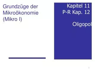
Grundzüge der Mikroökonomie (Mikro I) Kapitel 11 P-R Kap. 12 Oligopol Teil II
Stackelberg versus Cournot-Nash QA C QA+QH=100 100 Stackelberg Gleichgewicht: Der Stackelberg- Führer A wählt besten Punkt auf QH*(QA) 50 SE 37.5 33.3 QH* (QA)= 50 - 0.5QA NE QA*(QH)= BR(QH) = 50 - 0.5QH C QH 50 25 33.3 100 nicht „Rückverhandlungs-Stabil“: Wenn A nachfolgend ändern könnte
Preis- versus Mengenwettbewerb • Cournot-Wettbewerbmit 2 Anbietern: • Im Nash-Gleichgewichtwirdgrößere Menge als Monopolmenge bereitgestellt • Aber kleiner Menge als im Wettbewerbsmarkt • Preiswettbewerb mit homogenen Gütern (Bertrand) und vollkommen elastischem Angebot • wer den Preis des anderen um wenig unterbietet • erhält die ganze Nachfrage • Im Nash-Gw wird Preis = Grenzkosten realisiert
B A P=0,8 P=1 P=1 Bertrand-Wettbewerb (Intuition) P=0,8 QA=1,1,QB=1,1 PA=0,88;PA=0,88 QA=2,2,QB=0 PA=1,76;PA=0 QA=0,QB=2,2 PA=0;PA=1,76 QA=1,QB=1 PA=1;PB=1 Nachfragekurve P = 4 – Q, d.h. Marktnachfrage ist Q = 3 – P, MC = 0 Marktpreis P = Min (PA, PB) QA = Q wenn PA < PB QA = Q/2 wenn PA = PB QA = 0 wenn PA > PB
Preiswettbewerb mit heterogenen Gütern • Heterogene Güter • Unternehmen haben Marktmacht, d.h. verlieren nicht die gesamte Nachfrage wenn Preis den des Konkurrenten übersteigt • Im Nash-Gw ist PA> Grenzkosten von Aund PB> Grenzkosten von B • Preise bei Kartellbildung sind höher als Preise im Nash-Gw
Welches ist das richtige Wettbewerbsmodell? • Preiswettbewerb: • Preisvariable direkt unter Kontrolle der Unternehmen (Supermarkt) • Mengenwettbewerb • Unternehmen legen Kapazität im voraus fest • anschließend Preiswettbewerb • aber keine Anreize, ganze Marktnachfrage zu attrahieren wenn man sie ohnehin nicht bedienen kann
Themengebiete • Marktgleichgewicht (Kap. 2) • Präferenzen (Kap. 3) • Nachfrage (Kap. 4) • E‘ unter Unsicherheit (Kap. 5) • Tauschgleichgewicht (Kap. 6) • Produktions-und Kostentheorie (Kap. 7-9) • Monopol (Kap. 10) • Oligopol (Kap. 11) • 8 Teilgebiete • 5 Fragen • SIE: WÄHLEN 3
Musterklausur • Besprechung morgen • Lay-out wie Abschlussklausur • Reicht mit Sicherheit nicht zum Bestehen
Vorbereitung • nur Übung – nur Vorlesung? • auf die richtige Mischung kommt es an • Rechnen + Beherrschung der graphischen Darstellung
Beispiel • Cournot-Nash mit 2 Firmen mit steigenden Grenzkosten • C = ½( xi)2 • P=99 – x mit x = xA + xB • Residualnachfrage für A: • P= (99 – xB,fix) – xA Nash-Gleichgewicht des Cournotwettberbs
99 –2xA– xB,fix=xA (= MRA=MCA) • 99 – xB,fix=3xA • 33 – 1/3 xB,fix =xA
Cournot-Nash-Gleichgewicht xA C QA+QB=100 99 B‘s Reaktionskurve: xB*(xA)=BR(xA) = 33 - 1/3xA A‘s Reaktionskurve: xA* (xB)= BR(xB) = 33 - 1/3xB 33 C xB 33 99
Nash-Gleichgewichtsbedingung Nash-Gleichgewicht ist Paar xA* , xB*: xA*= BRA(xB*)) xB*= BRB(xA*) xA*= BRA( ) BRB( ) xA* Þ22 = (1 - 1/9) xA so xA=24.75 Þ xB=24.75
WelcheMengemaximiert den gemeinsamenGewinn? • PA+B = 99 (xA + xB) – (xA + xB)2 – ½ (xA)2 – ½ (xB)2 • dPA+B /dxA = 99 – 2 (xA + xB) – xA = 0, • dPA+B /dxB = 99 – 2 (xA + xB) – xB = 0. • xA = xB = 99/5 = 19,8 • oder: MR = MCA = MCB • xA = xB = x/2
Optimum füroptimaleAufteilungsregel • PA+B = 99 x – x2 – ½ (x/2)2 – ½ (x/2)2 • = 99 x – x2 – ¼ x2 • d PA+B/dx = 99 – 2 x – ½ x = 0 • MR(x)= MC(x) oder 99 – 2 x = ½ x • x = 99/2.5 = 39,6