Download
1 / 19
190 likes | 276 Views
This project aims to identify and rectify nonlinear errors affecting beam position spectra in the CESR accelerator. By investigating different methods through simulations and real-time testing, the goal is to enhance beam stability, minimize distortions, and optimize vertical bunch size. Learn about the impact of various magnets like dipoles, quadrupoles, and sextupoles in error detection and correction. Discover how Beam Position Monitors (BPMs) aid in monitoring beam positions. Explore methods involving Singular Value Decomposition and Sextupoles to analyze and resolve non-linear restoring forces. Dive into spectral components and eigenvalues to understand the relationship between driving amplitudes and harmonic signals. Examine the power law dependencies and tune shifts to enhance beam trajectory predictions. Unravel the impact of lattice changes on signal readings and devise strategies for error mitigation. This study aims to pave the way for more accurate and stable particle acceleration systems.

E N D
Searching for CesrTA guide field nonlinearities in beam position spectra Laurel Hales Mike Billing Mark Palmer
Goals • Learn how to find and correct non-linear errors. • Correcting these errors will allow us to • Withstand large amplitude oscillations without losing particles. • Get a small vertical bunch size and avoid bunch shape distortions. • We have two possible methods for finding non-linear errors. • Our first goal is to test these two methods using simulations. • Then we can test them using the accelerator.
Dipoles - Bend the beam. Quadrupoles - Focus the beam. Sextupoles - Compensate for the energy depended focusing due to the quadrupoles Errors in the optics can lead to: Losing particles Bunch shape distortions The optics
What is a BPM? • Beam Position Monitor inside the beam-pipe. • There are about 100 BPMs around CESR. • The BPM can give you an x position and a y position for the beam One BPM vs. Time Beam-pipe 4 electrodes on the walls of the beam-pipe
MIA • Drive beam with a sinusoidal shaker • Take position data: 100 BPMs ~ 1000 turns • Create a matrix P= [position x history] • Using Singular Value Decomposition to get: Columns = spatial function around ring (Diagonals) = Eigen values (λi) ~ amplitudes of the eigen components Columns = time development of beam trajectory
Our simulation • Our simulation uses tracking codes from BMAD. • In our simulation we give the particle bunch an initial amplitude and then track it as it circles freely. • There is no damping.
Sextupoles • Sextupoles have a non-linear restoring force: • which can be solved for: • when we solve the above equation that gives us different multiples of ω because:
1st Method One of the principle components • The height of the different harmonics should be dependent on the driving amplitude (A). Higher spectral component Τau matrix column
Results for Method 1 The expected power law dependence is clearly shown in the vertically driven simulation.
Machine data (horizontally driven) The horizontally driven data shows the power law relation between driving amplitude and the magnitude of the harmonic signals The line represents a linear dependence
Machine data (vertically driven) The vertically driven data also displays the power law relation. The line represents a linear dependence
β(s) is the amplitude function. β modulates the amplitude of the oscillation of the particle beam The envelope of oscillation is defined as , where J is the Action of the beam. Φ defines the phase of the oscillation. The phase increases monotonically but not uniformly The Φ and β of the ring will change when a quadrupole strength is changed. What are β and Φ?
x’ x x’ x 2nd Method • The sextupole magnets distort the phase space ellipse into a different shape. • This distortion changes the equilibrium value of β(s) • This change in β(s) is proportional to the driving amplitude: Without sextupoles With sextupoles
2nd Method • A change in β can create a change in phase. • The phase of the entire ring is the tune. The tune shift from the β error is: • We expect Q vs. A to have a parabolic relationship because:
Results for Method 2 The quadratic dependence is shown in the vertically driven simulation
Machine data The tune shift is large enough to see it in the data from the actual accelerator
A resonance? The horizontal data is not quite what we expected. This may be due to the fact that it is close to the 2(Qh)+3(Qv)+2(Qs)=3 or the 3(Qv)+3(Qs)=2 resonances.
Conclusions • We have shown that the magnitude for the signal heights of the different spectral components are dependent on the driving amplitude. • We have also shown that there is a tune shift that is dependent on the driving amplitude. • We have also shown that these effects can be detected in the signal from the particle accelerator.
Future plans • We need to determine how changing the lattice effects the signals. • From that data we can begin to figure out how we can use these methods to find non-linear errors.