Download
1 / 36
360 likes | 526 Views
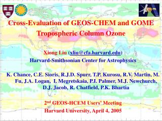
An Eight-Year Record of Ozone Profiles and Tropospheric Column Ozone from GOME. Xiong Liu, Kelly Chance, and Thomas Kurosu Harvard-Smithsonian Center for Astrophysics, Cambridge, MA, USA The 36 th COSPAR Scientific Assembly Beijing, China, July 19, 2006. Outline. Introduction

E N D
An Eight-Year Record of Ozone Profiles and Tropospheric Column Ozone from GOME Xiong Liu, Kelly Chance, and Thomas Kurosu Harvard-Smithsonian Center for Astrophysics, Cambridge, MA, USA The 36th COSPAR Scientific Assembly Beijing, China, July 19, 2006
Outline • Introduction • Examples of Retrievals • Algorithm Description • Retrieval Characterization • Intercomparison with TOMS, Dobson/Brewer, SAGE, and Ozonesonde Measurements • Summary and Future Outlook
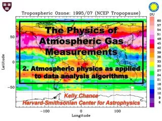
Introduction • Tropospheric O3: key species in air quality, climate, trop. chemistry • Chance et al. (1997): ozone profiles including tropospheric ozone can be derived from UV/Visible spectra(wavelength-dependent photon penetration and temperature-dependent Huggins bands) • GOME: April 1995, 240-790 nm, 0.2-0.4 nm FWHM, high SNR • Several other groups developed physically-based ozone profile algorithms: Munro et al., 1998; Hoogen et al., 1999, Hasekamp and Landgraf, 2001, van der A et al., 2002 • Tropospheric ozone retrievals remain challenging: consistent and accurate calibration, high fitting precision, 90% total ozone above • We recently developed our own ozone profile algorithm for GOME data and demonstrated that valuable tropospheric ozone can be derived from GOME (Liu et al., 2005, 2006a, 2006b, in press, 2006c submitted to ACP).
Examples of Retrievals (Ozone Profile) 24 ~2.5-km layers 4-6 tropospheric layers Ozone hole Biomass burning over Indonesia
Examples of Tropospheric Column Ozone (TCO) Three-day Comopsite Map (10/22-24/1997) Zonal contrast in the tropics Biomass burning over Indonesia
Algorithm Description • Fitting Windows: 289-307 nm, 325-340 nm, 368-372 nm (cloud) • Spatial resolution: 960 80 km2 • Spectral fitting + Optimal estimation + LIDORT • A Priori: ozone profile climatology by McPeters et al. [2003] • Measurement error: GOME random-noise error • Detailed treatments of wavelength and radiometric calibrations • Standard correction provided in GDP extraction software • Variable slit/wavelength calibration • Undersampling correction • Include a 2nd-order polynomial in the fitting in 289-307 nm • Derive degradation in reflectance: necessary for the 8-year record Liu et al., JGR, 2005
Algorithm Description Derive reflectance degradation: comparing averaged reflectance over 60ºN-60ºS to those in the first 6 months and removing SZA and seasonal dependent components Large degradation (up to 25%) and strong wavelength dependence Liu et al., submitted to ACP
Algorithm Description • LIDORT (pseudo-spherical) with additional corrections • Polarization correction • Ring effect:directly model the 1st-oder RRS of the direct beam • Clouds: Lambertian + IPA, GOMECAT CTP, fc from 368-372 nm • Aerosols:SAGE stratospheric and GOCART tropospheric • Surface albedo: varying with , initialized from an albedo database • NCEP surface & tropopause pressure, ECMWF temperature • Directly model and fit other trace gases: SO2, NO2, BrO, HCHO • NO2: PRATMO (stratosphere) + GEOS-CHEM (troposphere) • BrO: PRATMO (stratosphere) + well mixed in the troposphere • SO2/HCHO: no stratospheric + GEOS-CHEM (troposphere) • Use ozone cross section by Brion et al. [1993]: reduce residuals by 30-45% in the Huggins bands (vs. Bass-Paur and GOME FM) • Fitting residuals:< 0.1% in the Huggins bands (326-340 nm)
Retrieval Characterization --- Averaging Kernels 8-12 km (at 20-38 km) VR: 7-12 km (at 10-37 km) DFS:ranging from 1.2 in the tropics to 0.5 at high latitudes
Error Analysis Smoothing + Precision: TO: 3 DU (1.0%) SCO: 2-5 DU (1-2%) TCO: 3-6 DU (12-20%) Smoothing + Precision: 5-10% in the stratosphere & 20-30% in the troposphere
Total Column Ozone Comparison sonde+Dobson sonde only Comparisons with total ozone /ozonesonde at 33 sonde stations TOMS: mean biases are<6 DU (2%)at most stations with1 <1.5% in tropics and <2.4% at high latitudes Dobson:±8hrs, ±1.5ºlat, ±500km lon, mean biases are mostly<5 DU (2%)with1 < 3% in the tropics and <5% at high latitudes Liu et al., JGR, 2005
Comparison with Ozonesonde TCO 97-98 El Nino Event Java [110-125E, 6.6-8.6S] America Samoa [180-158E, 13.2-15.2S] Liu et al., JGR, 2006
Comparison with Ozonesonde TCO GOME TCO captures most of the temporal variability in ozonesonde TCO Mean biases:<3.3 DU (15%)at 30 stations 1 :3-8 DU (12-27%) Liu et al., JGR, 2005
Intercomparison with SAGE-II Comparisons with SAGE-II in 1996-1999 down to ~15 km: same day, ±1.5ºlat, ±5ºlon Systematic biases: usually <15% with 1 <10% at ~20-60 km Column ozone: <2.5 DU at ~15-35 km Liu et al., JGR, 2005, in press
Comparison with Ozonesonde and SAGE-II SCO Stratospheric column ozone between layer 4 and 7 (15~35 km) or between tropopause and layer 7 GOME/SONDE SCO (15-35 km): usually higher by 8-20 DU (5-8%) at CI & most tropical stations GOME/SAGE-II SCO (~15-35 km): usually within ±2.5 DU (1.5%) except for 3 Northern European stations Liu et al., JGR, in press
Profile Comparison with Ozonesonde and SAGE-II GOME/SAGE-II: usually <5% at layer 5 and 8-20% for layer 4 GOME/Sonde: mostly 5-20% for layer 5 and 20-60% for layer 4 GOME/sonde biases depends on sonde technique, sensor solution, and data processing, demonstrating the need to homogenize ozonesonde observations for reliable satellite validation Liu et al., JGR, in press
Summary and Future Outlook • Ozone profiles and tropospheric column ozone are retrieved from GOME spectra (289-307 nm, 325-340 nm) using the optimal estimation after extensive treatments of wavelength and radiometric calibrations and forward modeling • Retrieval have been extensively evaluated against TOMS, Dobson/Brewer, SAGE, and ozonesonde measurements. • An eight-year (July 1995-June 2003) record of ozone profiles (24-layers), total, stratospheric, and tropospheric column ozone from GOME is available. • Continue to improve the retrievals and apply this algorithm to SCIAMACHY, GOME-2, and OMI data. • Integrate with chemical transport model to understand global distribution of tropospheric ozone and its seasonal and interannual variability. • Tropospehric ozone budget and its radiative forcing
Thank you ! Acknowledgements • Supported by NASA and the Smithsonian Institution • ESA and DLR • TOMS, SAGE, WOUDC, SHADOZ, CMDL • NCEP, ECMWF, GEOS-CHEM, GOCART, PRATMO • Cluster machine and its support at Harvard-Smithsonian CFA
High Resolution Solar Reference Spectrum 0.01 nm with wavelength accurate to 0.002 nm (Caspar and Chance, 1997)
Variable Slit/Wavelength Calibration • Use GDP extraction software with all standard corrections • Instrument slit function characterization (Chance, 1998) • Assume Gaussian, use non-linear least squares fitting • High resolution solar reference spectrum (Caspar and Chance, 1998) • Variable slit widths (21 spectral pixels in 5-pixel increments)
0.27% 0.4% 0.1% Fitting Residuals
Effects of Ozone Cross Sections on Retrievals Total Column Ozone Tropospheric Column Ozone Ozone Profile
A Priori Influence (06/7-9/1997) TOMS V8 A Priori Retrieval with TOMS V8 A Priori GEOS-CHEM A Priori Retrieval with GEOS-CHEM A Priori
Informational Analysis --- DFS and A Priori Influence DFS:1.2 DFS in the tropics, 0.5 at high latitudes A Priori influence in TCO: 15% in the tropics, 50% at high-latitudes
Error Analysis Liu et al., 2005, JGR
Comparison with Ozonesonde Tropospheric Column Ozone • Mean biases: <3.3 DU (15%) at 30 stations; 1 : 3-8 DU (12-27%) • Improvements over a priori at most stations: either reduces MBs or 1 or increases the correlation
Comparison with Ozonesonde SCO 1%-KI buffered 2%-KI unbuffered • GOME SCO compares better with 1%-KI buffered than 2%-KI unbuffered by 11-16 DU. • Altitude-dependent total ozone normalization reduces the bias contrast and GOME/sonde biases mainly with 2%-KI unbuffered. http://www.cmdl.noaa.gov/infodata/ftpdata.html
Profile Comparison with Ozonesonde 50S/N 75S/N 30S/N 50S/N 0 30N • Systematic biases • Large positive biases of (30-70%) at Carbon Iodine and most tropical stations 30S 0
Profile Comparison with Ozonesonde • The biases relative to 1%-buffered is usually smaller by 5-15%. • Altitude-dependent homogenization reduces the bias with 2%-unbuffered. • Uncorrected altitude hysteresis can account for 5-15% biases.
GOME vs. GEOS-CHEM • Similar overall structures • Global biases: <2±4 DU, r=0.82-0.9 • SH: <1±2 DU,r=0.94-0.98 • NH: <4.3±4.6 DU, r=0.6-0.8
GOME vs. GEOS-CHEM • Usually within 5 DU. • Large positive bias of 5-15 DU at some northern tropical and subtropical regions:central America, tropical North Africa, Southeast Asia, Middle East