Download
1 / 9
90 likes | 104 Views
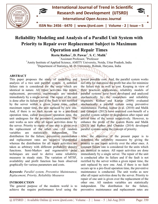
This paper proposes the study of modelling and analysis of a two unit parallel system. A constant failure rate is considered for the units which are identical in nature. All repair activities like repair, replacement, preventive maintenance are mended immediately by a single server. The repair of the unit is done after its failure and if the fault is not rectified by the server within a given repair time, called maximum repair time, the unit replaced by new one. And, if there is no fault occurs up to a pre fixed operation time, called maximum operation time, the unit undergoes for the preventive maintenance. The unit works as new after all repair activities done by the server. Priority to repair of one unit is given over the replacement of the other one. All random variables are statistically independent. The distribution for the failure, preventive maintenance and replacement rates are negative exponential whereas the distribution for all repair activities are taken as arbitrary with different probability density functions. Semi Markov and regenerative point techniques are used to derive some reliability measures in steady state. The variation of MTSF, availability and profit function has been observed graphically for various parameters and costs. Reetu Rathee | S. C. Malik | D. Pawar "Reliability Modeling and Analysis of a Parallel Unit System with Priority to Repair over Replacement Subject to Maximum Operation and Repair Times" Published in International Journal of Trend in Scientific Research and Development (ijtsrd), ISSN: 2456-6470, Volume-2 | Issue-5 , August 2018, URL: https://www.ijtsrd.com/papers/ijtsrd15655.pdf Paper URL: http://www.ijtsrd.com/mathemetics/statistics/15655/reliability-modeling-and-analysis-of-a-parallel-unit-system-with-priority-to-repair-over-replacement-subject-to-maximum-operation-and-repair-times/reetu-rathee<br>

E N D
International Research Research and Development (IJTSRD) International Open Access Journal Reliability Modeling and Analysis of a Parallel Unit Priority to Repair over Replacement Subject to Maximum Operation and Repair Times eetu Rathee1, D. Pawar1, S. C. Malik2 1Assistant Professor, 2Professor Amity Institute of Applied Science, AMITY University, Noida, Uttar Pradesh Department of Statistics, M. D. University, Rohtak, Haryana, India International Journal of Trend in Scientific Scientific (IJTSRD) International Open Access Journal ISSN No: 2456 ISSN No: 2456 - 6470 | www.ijtsrd.com | Volume 6470 | www.ijtsrd.com | Volume - 2 | Issue – 5 Reliability Modeling and Analysis of a Parallel Unit Priority to Repair o Operation and Repair Times Reetu Reliability Modeling and Analysis of a Parallel Unit System with Replacement Subject to Maximum 1Amity Institute of Applied Science, AMITY University, Noida 2Department of Statistics, M. Uttar Pradesh, India , India lowest possible cost. And, the parallel system works not only for maximize the profit but the failure risk as well as cost. their practical applications, reliability models of parallel systems have been developed and analyzed stochastically by the researchers and reliability engineers. Kishan and Kumar (2009 stochastically a parallel system using preventive maintenance. Further, kumar et al. (2010) and Malik and Gitanjali (2012) have analyzed cost parallel system subject to degradation after repair and arrival time of the server respec enhance the profit of the system (2013) and Rathee and Chander (2014) developed parallel systems using the concept of priority. Also, the objective of the present paper is to determine the reliability measures by giving priority to one repair activity over the other ones. A constant failure rate is considered for the units which are identical in nature. All repair activities are done immediately by a single server. The repair of the unit is conducted after its failure and if the fault is not rectified by the server within a given repair time, the unit replaced by new one. And, if there is no fault occurs up to a pre-fixed operation time, the preventive maintenance is conducted. The unit works as new after all repair activities done by the server. Priority to repair of one unit is given over the replacement of the other one. All random variables are statistically independent. The distribution for the failure, preventive maintenance and replacement rates are preventive maintenance and replacement rates are ABSTRACT This paper proposes the study of modelling and analysis of a two unit parallel system. A constant failure rate is considered for the units which are identical in nature. All repair activities like repair, replacement, preventive maintenance are mended immediately by a single server. The repair of the unit is done after its failure and if the fault is not rectified by the server within a given repair time, called maximum repair time, the unit replaced by new one. And, if there is no fault occurs up to a pre operation time, called maximum operation time, the unit undergoes for the preventive maintenance. The unit works as new after all repair activities done by the server. Priority to repair of one unit is given over the replacement of the other one. All random variables are statistically distribution for the failure, preventive maintenance and replacement rates are negative exponential whereas the distribution for all repair activities are taken as arbitrary with different probability density functions. Semi-Markov and regenerative point techniques are used to derive some reliability measures in steady state. The variation of MTSF, availability and profit function has been observed graphically for various parameters and costs. Keywords: Parallel system, Preventive Mai Replacement, Priority, Reliability Measures INTRODUCTION The general purpose of the modern world is to achieve the require performance level using the achieve the require performance level using the modelling and And, the parallel system works analysis of a two unit parallel system. A constant failure rate is considered for the units which are identical in nature. All repair activities like repair, replacement, preventive maintenance are mended not only for maximize the profit but also for minimize the failure risk as well as cost. Keeping in view of their practical applications, reliability models of parallel systems have been developed and analyzed stochastically by the researchers and reliability Kishan and Kumar (2009) evaluated stochastically a parallel system using preventive kumar et al. (2010) and Malik and Gitanjali (2012) have analyzed cost-benefit of a subject to degradation after repair and arrival time of the server respectively. However, to enhance the profit of the system Reetu and Malik (2013) and Rathee and Chander (2014) developed parallel systems using the concept of priority. repair of the unit is done after its failure and if the fault is not rectified by the server within a given repair time, called maximum repair time, the unit replaced by new one. And, if there is no fault occurs up to a pre-fixed ximum operation time, the unit undergoes for the preventive maintenance. The unit works as new after all repair activities done by the server. Priority to repair of one unit is given over the replacement of the other one. All random ally distribution for the failure, preventive maintenance and replacement rates are negative exponential whereas the distribution for all repair activities are taken as arbitrary with different probability density independent. independent. The The Also, the objective of the present paper is to determine the reliability measures by giving the priority to one repair activity over the other ones. A constant failure rate is considered for the units which are identical in nature. All repair activities are done immediately by a single server. The repair of the unit d regenerative point techniques are used to derive some reliability measures in steady state. The variation of MTSF, availability and profit function has been observed graphically for various parameters and costs. e and if the fault is not rectified by the server within a given repair time, the unit replaced by new one. And, if there is no fault fixed operation time, the preventive maintenance is conducted. The unit works as new ctivities done by the server. Priority to repair of one unit is given over the replacement of the other one. All random variables are statistically independent. The distribution for the failure, Parallel system, Preventive Maintenance, Measures The general purpose of the modern world is to @ IJTSRD | Available Online @ www.ijtsrd.com @ IJTSRD | Available Online @ www.ijtsrd.com | Volume – 2 | Issue – 5 | Jul-Aug 2018 Aug 2018 Page: 350
International Journal of Trend in Scientific Research and Development (IJTSRD) ISSN: 2456-6470 negative exponential whereas the distribution for all repair activities are taken as arbitrary with different probability density functions. Semi-Markov and regenerative point techniques are used to derive some reliability measures in steady state. The variation of MTSF, availability and profit function has been observed graphically for various parameters and costs. NOTATIONS: E : Set of regenerative states ?? : Set of non-regenerative states λ : Constant failure rate α0 : The rate by which system undergoes for preventive maintenance (called maximum constant rate of operation time) β0 : The rate by which system undergoes for replacement (called maximum constant rate of repair time) FUr /FWr : The unit is failed and under repair/waiting for repair FURp/FWRp : The unit is failed and under replacement/waiting for replacement UPm/WPm : The unit maintenance/waiting for preventive maintenance FUR/FWR : The unit is failed and under repair / waiting for repair continuously from previous state FURP/FWRP : The unit is failed and under /waiting for replacement continuously from previous state UPM/WPM : The unit is under/waiting for preventive maintenance continuously from previous state g(t)/G(t) : pdf/cdf of repair time of the unit f(t)/F(t) : pdf/cdf of preventive maintenance time of the unit r(t)/R(t) : pdf/cdf of replacement time of the unit qij (t)/Qij (t) : pdf / cdf of passage time from regenerative state Si to a regenerative stateSjor to a failed state Sj without visiting any other regenerative state in (0, t] qij.kr (t)/Qij.kr(t) : pdf/cdf of direct transition time from regenerative state Si to a regenerative state Sj or to a failed state Sj visiting state Sk, Sr once in (0, t] Mi(t) : Probability that the system up initially in state Si E is up at time t without visiting to any regenerative state Wi(t) : Probability that the server is busy in the state Si up to time ‘t’ without making any transition to any other regenerative state or returning to the same state via one or more non- regenerative states. i : The mean sojourn time in state ?? which is given by ∞ = ???? , ??= ?(?) = ? ?(? > ?) ?? ? is under preventive ? where?denotes the time to system failure. mij:Contribution to mean sojourn time (i) in state Si when system transits directlyto state Sjso that m and mij = i ij j *' ij tdQ t ( ) q (0) ij & */** : Symbol for Laplace Transformation /LaplaceStieltjes Transformation The states S0, S1, S2, S4, S6and S7 are regenerative while the states S3,S5, S8,S9, S10, S11 and S12 are non- regenerative as shown in figure 1. : Symbol for Laplace-Stieltjes convolution/Laplace convolution @ IJTSRD | Available Online @ www.ijtsrd.com | Volume – 2 | Issue – 5 | Jul-Aug 2018 Page: 351
International Journal of Trend in Scientific Research and Development (IJTSRD) ISSN: 2456-6470 TRANSITION STATE DIAGRAM Up-State λ 2λ FWr FUR O αO O S1 FUr SO O S2 Upm WPm S3 g(t) g(t) S5 βO f(t) f(t) βO FUR WPm αO f(t) r(t) S6 λ FWr UPM O UPm βO λ FUr FWRp O FURp S10 g(t) S11 FURp WPM S7 S4 αO r(t) r(t) αO f(t) βO g(t) r(t) FURp FWRP UPM WPm WPm FURP S8 S12 S9 Failed-State Regenerative point Fig. 1 Transition Probabilities and Mean Sojourn Times Simple probabilistic considerations yield the following expressions for the non-zero elements 0 2 2 0 2 0 ( g , 26 84 96 10,6 p p p p It can be easily verify that p p p p p p p p p p p p p p p p p ( p Q ) q ( t ) dt as (1) ij ij ij * 0 0 , , p p p (1 g ( )), 15 0 0 01 02 ) 0 0 * * * r p ( ), , p f ( ), p (1 g ( )) 40 0 13 0 0 60 0 ( ) 0 0 * * * g p ( ), , 17.3 p (1 g ( ))(1 g ( )) 10 0 0 0 0 0 ( ) 0 0 * * 0 , , 6,12 p 66.12 p (1 f ( )) 6,11 p 61.11 p (1 f ( )) 0 0 ( ) ( ) 0 0 * * 0 g p 5,10 p p 74.8 p 1 ( ) , , p p (1 r ( )) 37 78 0 49 46.9 0 ( ) 0 * * 0 , , p (1 g ( )) p (1 r ( )) 14 0 0 47 0 ( ) ( ) 0 p 0 0 * p p ( ) 11,1 p 12,6 p 1 31 56 74 0 p p 6,11 p 6,12 p 1 01 02 10 13 14 15 26 40 47 49 p 60 1 10 14 11.3 p 16.5 16.5,10 p 17.3 1 40 47 46.9 p 61.11 p p 60 66.12 74 74.8 @ IJTSRD | Available Online @ www.ijtsrd.com | Volume – 2 | Issue – 5 | Jul-Aug 2018 Page: 352
International Journal of Trend in Scientific Research and Development (IJTSRD) ISSN: 2456-6470 The mean sojourn times (??) is in the state Si are 02, m m 1 10 m ' 1 10 14 11.3 16.5 m m m m ' 4 40 47 m m m 7 Reliability and Mean Time to System Failure (MTSF) Let i(t) be the cdf of first passage time from regenerative state Si to a failed state. Regarding thefailed state as absorbing state, we have the following recursive relations for i(t): ( ) ( ( ) ) ( ) t Q t t Q t & ( ) ( ( ) ( ) ( ) ( ) ) ( ) t Q t t t Q Q t t t Q & & ( ) ( ) ( ) ( ) ( ) t t Q t Q t Q t & Taking LST of above relation (7.4) and solving for Ф? ** * 1 ( ) ( ) R s s The reliability of the system model can be obtained by taking Inverse Laplace transform of (3). The mean time to system failure (MTSF) is given by ** 1 ( ) lim s s D Where N p p p and 01 10 01 14 40 1 D p p p p p Steady State Availability Let Ai(t) be the probability that the system is in up-state at instant ‘t’ given that thesystementered regenerative state Si at t = 0.The recursive relations for ( ) ( ) ( ) ( ) ( ) ( ) ( ) A t M t q t A t q t A t ( ) ( ) ( ) ( ) ( ) ( ) ( ) ( ) ( ) ( ( ) ( )) ( ) q t A t q t q t A t ( ) ( ) ( ) A t q t A t ( ) ( ) ( ) ( ) ( ) ( ) ( ) A t M t q t A t q t A t q t A t ( ) ( ) ( ) ( ) ( ) ( ) ( ) A t M t q t A t q t A t q t ( ) ( ( ) ( )) ( ) A t q t q t A t Where (2 ) 0( ) , M t e ( ) , M t e G t ( ) 4( ) ( ) , M t e R t ( ) M t e F t Taking LT of above relation (6) and solving for A0*(s). The steady state availability is given by N A sA s D Where [(1 ){ (1 ) } ( [(1 ){ ( ) (1 )} p p p p p p m m m 15, m m 26, m m m 49, m m 6,12, m 0 01 13 14 2 4 40 47 6 60 6,11 16.5,10 m m 17.3, 46.9, 74.8, m 74 0 01 1 02 1 10 0 14 4 13 15 (2) 4 4 0 0 48 4 9 ∗∗(s), we have s (3) s N MTSF = (4) 0 (5) 0 01 1 01 14 4 iA t are given as: 0 0 01 1 02 2 A t A t M t q t A t 11.3 q t q t A t ( ) 1 1 10 0 1 14 4 17.3 7 16.5 16.5,10 6 2 26 6 ( ) A t ( ) 4 4 40 0 47 7 46.9 6 6 6 60 0 61.11 1 66.12 6 (6) 7 74 74.8 4 t ( ) t 1( ) 0 0 0 t ( ) t (7) 6( ) 0 0 * 0 1 ( ) (8) lim s ( ) 0 0 1 N p p 11.3 p 61.11 10 p p 61.11 40 p p p 17.3 p )] 1 0 47 60 14 6 47 ( 01 16.5 )] 16.5,10 (1 p 02 p 11.3 p (9) p p p 17.3 p p p p ){ (1 ) 02 61.11 p p } 01 46.9 ( p 14 1 47 } 01 66.12 17.3 p ){ 4 14 01 60 61.11 @ IJTSRD | Available Online @ www.ijtsrd.com | Volume – 2 | Issue – 5 | Jul-Aug 2018 Page: 353
International Journal of Trend in Scientific Research and Development (IJTSRD) ISSN: 2456-6470 D ( 2 02 p p )[(1 p ){ p (1 p ) p p } 61.11 40 p p p p ( p 17.3 p p )] 1 0 47 p 60 11.3 ) 61.11 10 (1 14 p ' [(1 ){ p ( 16.5,10 p p 11.3 p )} ( )] 6 47 01 16.5 ' 4 p 02 ' 7 01 46.9 14 17.3 (10) ( p p p ){ ( p 17.3 p p p ) ( 14 47 p p 17.3 p )} 01 60 (1 61.11 ){ p 14 ' p ( 1 ) } 1 47 01 66.12 02 61.11 Busy Period Analysis for Server A. Due to Repair Let ( ) iB t be the probability that the server is busy in repairof the unit at an instant‘t’ given that the system entered regenerative state Si at t=0.The recursive relations for R R iB ( ) t are as follows: R R R B ( ) t q ( ) t B ( ) t q ( ) t B ( ) t 0 R 01 1 02 R 2 R R B ( ) t W t ( ) q ( ) t B ( ) t q ( ) t B ( ) t q ( ) t B ( ) t 1 1 q 10 0 11.3 ( ) t 1 14 B 4 R R ( ) t B ( ) t ( 16.5 q 16.5,10 q ( )) t ( ) t 17.3 7 6 R R B ( ) t q ( ) t B ( ) t 2 R 26 6 R R R B ( ) t q ( ) t B ( ) t q ( ) t B ( ) t q ( ) t B ( ) t 4 R 40 0 R 47 7 46.9 q 6 R R B ( ) t q ( ) t B ( ) t 61.11 q q ( ) t B ( ) t ( ) t B ( ) t 6 R 60 0 1 66.12 6 R B Where, ( ) W t ( ) t W t ( ) ( q ( ) t ( )) t B ( ) t (11) 7 7 74 74.8 4 ( ) t ( ) t ( ) t 1) ( ) ( G t 1) ( ) G t e ( ) ( G t e e 0 0 0 0 0 0 1 0 t 0 W t ( ) e G t ( ) and (12) s .The time for which serveris busydue to repair is given 7 R * Taking LT of above relation (11) and solving for by N B sB s D Where , * 2 1 47 01 (0)(1 ){ (1 N W p p and D1 is already mentioned. B. Due to Replacement Let ( ) iB t be the probability that the server is busy in replacement of the unit at an instant ‘t’ given that the system entered regenerative state Si at t=0.The recursive relations for 0( ) B R R * 2 ( ) (13) ( ) lim s 0 0 0 1 * 66.12 p ) p p } W (0)( p p 17.3 p ){ 01 60 p p 61.11 p } 02 61.11 7 14 47 (14) Rp Rp iB ( ) t are as follows: Rp Rp Rp B ( ) t q ( ) t B ( ) t q ( ) t B ( ) t 01 02 0 Rp 1 2 B Rp Rp Rp B ( ) t q ( ) t B ( ) t 11.3 q ( ) t ( ) t q ( ) t B ( ) t 10 14 1 0 1 4 Rp Rp 17.3 q ( ) t B ( ) t ( 16.5 q ( ) t 16.5,10 q ( )) t B ( ) t 7 ( ) t 6 Rp Rp B ( ) t q ( ) t B 26 2 Rp 6 Rp Rp Rp B ( ) t W t ( ) q ( ) t B ( ) t q ( ) t B ( ) t q ( ) t B ( ) t 4 40 Rp B 47 46.9 ( ) t 7 4 Rp 0 q 6 Rp Rp B ( ) t q ( ) t ( ) t ( ) t B ( ) t 66.12 q B ( ) t 60 q 61.11 B 6 Rp 0 q 1 6 Rp B Where, ( ) t ( ( ) t ( )) t ( ) t (15) 74 74.8 7 4 @ IJTSRD | Available Online @ www.ijtsrd.com | Volume – 2 | Issue – 5 | Jul-Aug 2018 Page: 354
International Journal of Trend in Scientific Research and Development (IJTSRD) ISSN: 2456-6470 ( ) t ( ) t 1) ( ) R t W t ( ) e ( ) ( R t e (16) 0 0 4 0 Rp * Taking LT of above relation (15) and solving for is given by B ( ) s .The time for which server is busy due to replacement 0 N D Rp Rp * 3 ( ) (17) B sB ( ) s lim s 0 0 0 1 Where, N C. Due to Preventive Maintenance Let ( ) iB t be the probability that the server is busy in preventive maintenance of the unit at an instant‘t’ given that the system entered regenerative state Si at t=0.The recursive relations for * W (0)( p 17.3 p )( 01 60 p p 61.11 p ) and D1 is already mentioned. (18) 3 4 14 P P iB ( ) t are as follows: P P P B ( ) t q ( ) t B ( ) t q ( ) t B ( ) t 0 P 01 1 P 02 2 B P P B ( ) t q ( ) t B ( ) t 11.3 q t ( ) t ( ) t q ( ) t B ( ) t 1 10 0 1 14 4 P P 17.3 q ( ) t B ( ) ( 16.5 q ( ) t 16.5,10 q ( )) t B ( ) t 7 6 P P B ( ) t W t ( ) q ( ) t B ( ) t 2 P 2 26 P 6 P P B ( ) t q ( ) t B ( ) t q ( ) t B ( ) t q ( ) t B ( ) t 4 P 40 0 47 P 7 46.9 B 6 P P B ( ) t W t ( ) q ( ) t B ( ) t 61.11 q ( ) t ( ) t ( ) t 66.12 q ( ) t B ( ) t 6 P 6 60 q 0 1 6 P B Where, ( ) W t ( ) t ( q ( ) t ( )) t B (19) 7 74 74.8 4 ( ) t ( ) t ( ) t 1) ( ) ( F t 1) ( ) F t W t 2( ) F t ( ) e ( ) ( F t e e and (20) 0 0 0 6 0 P * Taking LT of above relation (19) and solving for maintenance is given by N B sB s D Where, * 4 2 02 47 * 6 47 (0)[(1 ){ W p p and D1 is already mentioned. Expected Number of Repairs Let ( ) iR t be the expected number of repairs by the server in (0, t] given that the system entered the regenerative state Si at t = 0. The recursive relations for ( ) iR t are given as: ( ) ( ) ( ) ( ) ( ) R t Q t R t Q t R t & & ( ) ( ) [1 ( )] ( ) [1 ( )] ( ) ( ) ( ) ( ) [1 ( )] ( ) Q t R t Q t R t Q & & ( ) ( ) ( ) R t Q t R t & ( ) ( ) ( ) ( ) ( ) ( ) ( ) R t Q t R t Q t R t Q t R t & & & ( ) ( ) ( ) ( ) ( ) ( ) ( ) R t Q t R t Q t R t Q t R t & & & ( ) ( ) [1 ( )] ( ) ( ) R t Q t R t Q t R t & & 0( ) B s .The time for which server is busy due to preventive P P * 4 ( ) (21) ( ) lim s 0 0 0 1 N W (0) p [(1 p ){ p (1 11.3 p ) p p } 61.11 p p p ( p 17.3 p )] 60 ( 61.11 10 ) p 40 )} 14 p p 16.5 p 16.5,10 p (1 ( p 17.3 p )] 01 02 11.3 01 46.9 14 (22) 0 01 1 02 2 t R t Q t & R t 11.3 Q & R t Q t & R t & ( ) R t 1 10 0 1 14 4 t ( ) 17.3 7 16.5 6 16.5,10 6 2 26 6 4 40 0 47 7 46.9 6 6 60 0 61.11 1 66.12 6 (23) 7 74 4 74.8 4 @ IJTSRD | Available Online @ www.ijtsrd.com | Volume – 2 | Issue – 5 | Jul-Aug 2018 Page: 355
International Journal of Trend in Scientific Research and Development (IJTSRD) ISSN: 2456-6470 ** 0( ) R Taking LST of above relations (23) and solving for server are giving by N R sR s D Where, ( )(1 ( )( p p p p and D1 is already mentioned. Expected Number of Replacements Let ( ) i Rp t be the expected number of replacements by the server in (0, t] given that the system entered the regenerative state Si at t = 0. The recursive relations for ( ) ( ) ( ) ( ) ( ) Rp t Q t Rp t Q t Rp t & & ( ) ( ) ( ) ( ) ( ) ( ) ( ) ( ) ( ) [1 ( )] Q t Rp t Q t Rp t Q & & ( ) ( ) ( ) Rp t Q t Rp t & ( ) ( ) [1 ( )] ( ) ( ) ( ) Rp t Q t Rp t Q t Rp t Q t & & ( ) ( ) ( ) ( ) ( ) ( ) Rp t Q t Rp t Q t Rp t Q t & & & ( ) ( ) ( )] ( ) [1 ( )] Rp t Q t Rp t Q t Rp t & & Taking LST of above relations (26) and solving for 0( ) Rp the server are giving by N Rp sRp s D Where, (1 ){ (1 ) } N p p p p p p and D1 is already mentioned. Expected Number of Preventive Maintenances Let ( ) iP t be the expected number of preventive maintenance by the server in (0, t] given that the system entered the regenerative state Siat t = 0. The recursive relations for ( ) ( ) ( ) ( ) ( ) ( ) P t Q t P t Q t P t & & ( ) ( ) ( ) ( ) ( ) ( ) ( ) ( ) ( ) { ( ) ( )} ( ) Q t P t Q t Q t P t & & ( ) ( ) [1 ( )] P t Q t P t & ( ) ( ) ( ) ( ) ( ) ( ) ( ) P t Q t P t Q t P t Q t P t & & & ( ) ( ) [1 ( )] ( ) [1 ( )] P t Q t P t Q t P t Q & & ( ) { ( ) ( )} ( ) P t Q t Q t P t & Taking LST of above relations (29) and solving for 0( ) P unit time by the server are giving by s .The expected no. of repairs per unit time by the ** 0 5 ( ) (24) ( ) lim s 0 0 1 N p 11.3 p 16.5 p p ){ p (1 p ) p p } 5 10 47 01 66.12 ) 02 61.11 p p 61.11 p 74 14 47 17.3 01 60 (25) Rp t are given as: ( ) i 0 01 1 02 2 Rp t Q t & Rp t 11.3 Q t & Rp t Q t & Rp t ( ) 1 10 0 1 14 4 ( ) t & Rp t ( ) 17.3 7 16.5,10 6 16.5 6 2 26 6 & Rp t [1 Rp t ( ) ( )] 4 40 0 47 7 46.9 6 6 60 0 61.11 1 66.12 6 (26) 7 74 4 74.8 4 ** s .The expected no. of replacements per unit time by ** 0 6 ( ) (27) ( ) lim s 0 0 1 6 16.5,10 ( p p 47 01 66.12 02 61.11 46.9 )( p p p p p 17.3 p p p ){ p p 61.11 p } 40 14 01 p 60 ( 17.3 p )( ) 74.8 14 47 01 60 61.11 (28) iP t are given as: 0 01 1 02 2 P t P t Q t & P t 11.3 Q t & Q t & P t 1 10 0 1 14 4 17.3 7 16.5 16.5,10 6 2 26 6 4 40 0 47 7 46.9 6 ( ) [1 t & P t ( )] 6 60 0 61.11 1 66.12 6 (29) 7 74 74.8 4 ** s .The expected no. of preventive maintenances per @ IJTSRD | Available Online @ www.ijtsrd.com | Volume – 2 | Issue – 5 | Jul-Aug 2018 Page: 356
International Journal of Trend in Scientific Research and Development (IJTSRD) ISSN: 2456-6470 N D ** 0 7 ( ) (30) P lim s sP ( ) s 0 0 1 Where, N p [(1 p ){ p p (1 11.3 p ) p p } 61.11 p p p ( p p p p )] 7 02 [(1 47 ){ 60 ( 61.11 10 ) p 40 14 17.3 ( p p 16.5 p 16.5,10 p (1 )} 17.3 p )] 47 01 02 11.3 01 46.9 14 and D1 is already mentioned. Profit Analysis The profit incurred to the system model in steady state can be obtained as R Rp P K A K B K B K B K R P Where, P = Profit of the system model after reducing cost per unit time busy of the server and cost per repair activity per unit time K = Revenue per unit up-time of the system K =Cost per unit time for which server is busy due to repair K =Cost per unit time for which server is busy due to replacement K =Cost per unit time for which server is busy due to preventive maintenance K = Cost per repair per unit time K = Cost per replacement per unit time K = Cost per preventive maintenance per unit time CONCLUSION After solving the equations of MTSF, availability and profit function for the particular case g(t) = ?????, r(t) = ????? and f(t) = ?????, we conclude that These reliability measures are increasing as the repair rate θ, replacement rate β increases while their values decline with the increase of failure rate λ and the rate ?? by which the unit undergoes for preventive maintenance. The MTSF and availability keep on upwards with the increase of the rate ?? by which unit undergoes for replacement but profit decreases. The system model becomes more profitable when we increase the preventive maintenance rate α. GRAPHS FOR PARTICULAR CASE MTSF Vs Failure Rate (λ) (31) K R p K 6 0 P (32) 0 0 1 0 2 0 3 0 4 1 5 0 0 1 2 3 4 5 6 5.02 α0=0.2,β0=3,θ=2.1,α=5,β=10 β0=1 θ=4.1 α0=0.201 α=7 β=5 5 4.98 4.96 4.94 4.92 MTSF 4.9 4.88 4.86 0.01 0.02 0.03 0.04 0.05 0.06 0.07 0.08 0.09 Failure Rate (λ) Fig.2 @ IJTSRD | Available Online @ www.ijtsrd.com | Volume – 2 | Issue – 5 | Jul-Aug 2018 Page: 357
International Journal of Trend in Scientific Research and Development (IJTSRD) ISSN: 2456-6470 Availability Vs Failure Rate (λ) 0.973 0.971 α0=0.2,β0=3,θ=2.1,α=5,β=10 β0=1 θ=4.1 α0=0.201 α=7 β=5 0.969 0.967 0.965 0.963 Availability 0.961 0.959 0.957 0.955 0.01 0.02 0.03 0.04 0.05 0.06 0.07 0.08 0.09 Failure Rate (λ) Fig.3 Profit Vs Failure Rate (λ) 13950 13850 α0=0.2,β0=3,θ=2.1,α=5,β=10 β0=1 θ=4.1 α0=0.201 α=7 β=5 13750 13650 13550 13450 13350 Profit (P) 13250 13150 13050 0.01 0.02 0.03 0.04 0.05 0.06 0.07 0.08 0.09 Failure Rate (λ) Fig.4 REFERENCES 1.R. Kishan and M. Kumar (2009), “Stochastic analysis of a two-unit parallel system with preventive maintenance”, Journal of Reliability and Statistical Studies, vol. 22, pp. 31- 38. 4.Reetu and Malik S.C. (2013),A Parallel System with Priority to Preventive Maintenance Subject to Maximum Operation and Repair Time. American journal of Mathematics and Statistics, Vol. 3(6), pp. 436-440. 2.Kumar, Jitender, Kadyan, M.S. and Malik, S.C. (2010): Cost-benefit analysis of a two-unit parallel system subject to degradation after repair. Journal of Applied Mathematical Sciences, Vol.4 (56), pp.2749-2758. 5.Rathee R. and Chander S. (2014), A Parallel System with Priority to Repair over Preventive Maintenance Subject to Maximum Operation and Repair Time. International Journal of Statistics and Reliability Engineering, Vol. 1(1), pp. 57-68. 3.Malik S.C. and Gitanjali (2012). Cost-Benefit Analysis of a Parallel System with Arrival Time of the Server and Maximum Repair Time. International Journal of Computer Applications, 46 (5): 39-44. @ IJTSRD | Available Online @ www.ijtsrd.com | Volume – 2 | Issue – 5 | Jul-Aug 2018 Page: 358