Download
1 / 9
90 likes | 111 Views
This paper explored four models in determining the impact of four agricultural sub-sectors of on the Nigerian GDP. The data is on the contribution of four different sub-sectors of agriculture on Nigerian Economy and was obtained from Central Bank of Nigeria statistical bulletin. The findings revealed that ridge regression and PCR are good regression estimation methods for predicting GDP. From the models there is strong indication that fish production in Nigeria is too insufficient to sustain her ever increasing population and improve her economy. Also, the ever increasing demand for fish by Nigerians due to high cost of meat in the market is clearly shown in the models and this stands to say that a lot need to be done to improve fish production in Nigeria to ensure sustainable growth and development. Okeke, Evelyn Nkiruka | Okeke, Joseph Uchenna"Exploratory Model of the Impact of Agriculture on Nigerian Economy" Published in International Journal of Trend in Scientific Research and Development (ijtsrd), ISSN: 2456-6470, Volume-1 | Issue-4 , June 2017, URL: http://www.ijtsrd.com/papers/ijtsrd162.pdf http://www.ijtsrd.com/economics/development-economics/162/exploratory-model-of-the-impact-of-agriculture-on-nigerian-economy/okeke-evelyn-nkiruka<br>

E N D
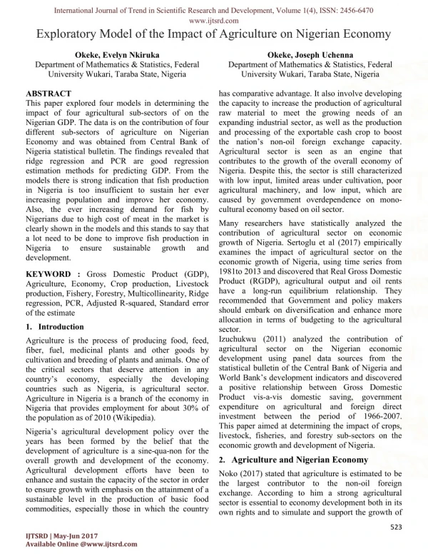
International Journal of Trend in Scientific Research and Development, Volume 1(4), ISSN: 2456-6470 www.ijtsrd.com Exploratory Model of the Impact of Agriculture on Nigerian Economy Okeke, Evelyn Nkiruka Department of Mathematics & Statistics, Federal University Wukari, Taraba State, Nigeria ABSTRACT This paper explored four models in determining the impact of four agricultural sub-sectors of on the Nigerian GDP. The data is on the contribution of four different sub-sectors of agriculture on Nigerian Economy and was obtained from Central Bank of Nigeria statistical bulletin. The findings revealed that ridge regression and PCR are good regression estimation methods for predicting GDP. From the models there is strong indication that fish production in Nigeria is too insufficient to sustain her ever increasing population and improve her economy. Also, the ever increasing demand for fish by Nigerians due to high cost of meat in the market is clearly shown in the models and this stands to say that a lot need to be done to improve fish production in Nigeria to ensure sustainable development. Okeke, Joseph Uchenna Department of Mathematics & Statistics, Federal University Wukari, Taraba State, Nigeria has comparative advantage. It also involve developing the capacity to increase the production of agricultural raw material to meet the growing needs of an expanding industrial sector, as well as the production and processing of the exportable cash crop to boost the nation’s non-oil foreign exchange capacity. Agricultural sector is seen as an engine that contributes to the growth of the overall economy of Nigeria. Despite this, the sector is still characterized with low input, limited areas under cultivation, poor agricultural machinery, and low input, which are caused by government overdependence on mono- cultural economy based on oil sector. Many researchers have statistically analyzed the contribution of agricultural sector on economic growth of Nigeria. Sertoglu et al (2017) empirically examines the impact of agricultural sector on the economic growth of Nigeria, using time series from 1981to 2013 and discovered that Real Gross Domestic Product (RGDP), agricultural output and oil rents have a long-run equilibrium relationship. They recommended that Government and policy makers should embark on diversification and enhance more allocation in terms of budgeting to the agricultural sector. Izuchukwu (2011) analyzed the contribution of agricultural sector on the Nigerian economic development using panel data sources from the statistical bulletin of the Central Bank of Nigeria and World Bank’s development indicators and discovered a positive relationship between Gross Domestic Product vis-a-vis domestic saving, government expenditure on agricultural and foreign direct investment between the period of 1966-2007. This paper aimed at determining the impact of crops, livestock, fisheries, and forestry sub-sectors on the economic growth and development of Nigeria. growth and KEYWORD : Gross Domestic Product (GDP), Agriculture, Economy, Crop production, Livestock production, Fishery, Forestry, Multicollinearity, Ridge regression, PCR, Adjusted R-squared, Standard error of the estimate 1.Introduction Agriculture is the process of producing food, feed, fiber, fuel, medicinal plants and other goods by cultivation and breeding of plants and animals. One of the critical sectors that deserve attention in any country’s economy, especially the developing countries such as Nigeria, is agricultural sector. Agriculture in Nigeria is a branch of the economy in Nigeria that provides employment for about 30% of the population as of 2010 (Wikipedia). Nigeria’s agricultural development policy over the years has been formed by the belief that the development of agriculture is a sine-qua-non for the overall growth and development of the economy. Agricultural development efforts have been to enhance and sustain the capacity of the sector in order to ensure growth with emphasis on the attainment of a sustainable level in the production of basic food commodities, especially those in which the country 2.Agriculture and Nigerian Economy Noko (2017) stated that agriculture is estimated to be the largest contributor to the non-oil foreign exchange. According to him a strong agricultural sector is essential to economy development both in its own rights and to simulate and support the growth of 523 IJTSRD | May-Jun 2017 Available Online @www.ijtsrd.com
International Journal of Trend in Scientific Research and Development, Volume 1(4), ISSN: 2456-6470 www.ijtsrd.com industries. Economy growth has gone hand in hand with agricultural progress; stagflation in agriculture is the principal explanation for poor economy performance, while rising agricultural activities has been the most concomitant of successful industrialization (Ukeje 1999). The labour-intensive character of the sector reduces its contribution to the GDP; Noko lamented, and still maintained that agricultural exports are a major earner of foreign exchange in Nigeria. in 1980 to 20%, and 19% in 1985 which was as a result of oil glut of the 1980’s. Historically, the root of the crisis in Nigeria economy lies in the neglects of the agricultural sector by the Federal Government of Nigeria due to oil sector. The GDP from agriculture decreased to 4,662,010.12 NGN million in the fourth quarter of 2016 from 5,035,069.07 NGN millions in the third quarter of 2016. GDP from agriculture in Nigeria averaged 369,673.12NGN million from 2010 until 2016, reaching an all time high of 5,035,069.07NGN in the third quarter of 2016 and a record low of 2,594,759.86NGN million in the first quarter of 2010 (CBN 2014). Below is the Table showing the GDP from Agriculture and other sources In an effort to increase the agricultural production in Nigeria, this year, 2017, the Central Bank of Nigeria has approved the disbursement of about #75 billion as loan to farmers in the 36 states and the Federal Capital Territory (FCT) under the Nigerian Incentive-Based Risk Sharing in Agricultural Lending (NIRSAL). The loan guarantee scheme is a public-private sector initiative set up to transform the country’s agricultural sector. It was initiated by the Apex bank, the Banker’s Committee and the Federal Ministry of Agriculture and rural Development, to guarantee 75% loans provided by Deposit Money Banks to farmers as part of effort to transform the countries agricultural sector (Uzonwanne 2017) Table 1: Distribution of Last and Previous Quarter of 2013 GDP from Agriculture and Others Last Quarter of 2013 4,662,010.12 623,349.23 1,645,401.74 2,041,492.97 Previous Quarter 5,035,069.07 543,808.12 1,614,894.65 1,624,018.01 GDP Agriculture Construction Manufacturing Mining Public Administration Services Transport Utilities Source: National Bureau of Statistics Gollin et al (2004) emphasized that low agricultural productivity can substantially delay industrialization. According to them improvement in the agricultural productivity can hasten the start of industrialization and hence have large effects on a country’s relative income. It provides employment opportunities for the teeming population, eradicates contributes to the growth to the economy. 430,861.50 371,731.33 6,977,150.10 217,313.24 111,801.06 6,035,650.62 210,972.66 85,432.68 poverty and Ukeji (2003) submitted that in the 1960’s agriculture contributed up to 64% to the nation’s total GDP but it gradually declined to 48% in 1970’s and it continued Fig 1: Last and Previous Quarter of 2016 GDP from Agriculture and Others 8000000 7000000 6000000 5000000 4000000 3000000 2000000 Last Quarter of 2016 1000000 0 Previous Quarter 524 IJTSRD | May-Jun 2017 Available Online @www.ijtsrd.com
International Journal of Trend in Scientific Research and Development, Volume 1(4), ISSN: 2456-6470 www.ijtsrd.com In 1990, policy measures were initialized and strategies designed to propel agricultural development targeting the year 2010. Emphasis was on food, livestock, the fisheries and the forestry. from such plants preserved and they include: timber for plywood, furniture, manufacturing of papers, electric poles etc. houses and boats, Fishing sub-sector involves breeding and catching fishes from the rivers for human consumption. Fishing constitutes major occupation of river line people. Fish constitute main sources of protein. Ezeokoli (2011) Food crops constitute the largest component of crops sub-sector of Nigeria’s agricultural sector. They are categorized broadly into cereals, roots, tubers, plantain, oil seeds and nuts, pulses, vegetables and fruits, sugar and beverages. 3.Data and its Presentation The data used for this work is mainly secondary data, sourced from the Central Bank of Nigeria statistical bulletin (2014) via: annual report and statement of account. Information on the annual GDP from agricultural sub-sector: food crop production (??), livestock production (??), forestry (??), fishing (??) and total GDP (Y) were collected for analysis. The period covered is 33 years from 1981to 2013. Below is the contribution of agricultural sector to total GDP for the period of 32 years. For the purpose of planning of self-sufficiency in livestock production, output in the sector has been categorized into short and long term. Livestock whose sufficiency level could be conveniently attained within five years such as beef, poultry products, goat meat, mutton, and pork were classified as short term while those that would at least in 15years be sufficient were categorized as long term. Forestry concern is on the preservation and maintenance of economic trees and plants. It also involves the eradication of various forms of resources associated with forest. Agriculturists derived a lot Agriculture 16000 14000 12000 10000 8000 Agriculture 6000 4000 2000 0 1970 1980 1990 2000 2010 2020 Fig. 2: Annual GDP from Agriculture from 1981to 2013 525 IJTSRD | May-Jun 2017 Available Online @www.ijtsrd.com
International Journal of Trend in Scientific Research and Development, Volume 1(4), ISSN: 2456-6470 www.ijtsrd.com 45000 40000 35000 30000 25000 Total GDP 20000 Agriculture 15000 10000 5000 0 1 3 5 7 9 11 13 15 17 19 21 23 25 27 29 31 33 Fig. 3: Bar chart of Total GDP and GDP from Agriculture The graphical display of four quarters of 2013 data is presented in figure 3 below to give us an overview of each sub-sectors contribution to the entire GDP from Agriculture. 5000 4500 4000 3500 3000 Q1 2500 Q2 2000 Q3 1500 Q4 1000 500 0 Agriculture Crop Livestock Forestry Fishing production Fig. 2: Quarterly Gross Domestic Product at Current Basic Price (N’ Billion) for 2013 To determine the suitable model we are going to build for our data, the correlation matrix for the data was computed to check for possible correlates. The correlation matrix for the data is shown in Appendix A below. multiple regressions. Suppose we have the sum of four explanatory variables ??+ ??+ ??+ ??as in the case of this our study as a component of a whole, then there is tendency that the variables will be linearly related to one another, thereby creating inaccurate estimate of the regression coefficients. Observe from the correlation matrix in Appendix A that there exists perfect linear relationship between crop production and livestock and near perfect relationship among other variables. This is a case of data that is suffering from multicollinearity. When the 4.Methodology 4.1 Collinearity Collinearity is the existence of near perfect linear relationship among the explanatory variables of 526 IJTSRD | May-Jun 2017 Available Online @www.ijtsrd.com
International Journal of Trend in Scientific Research and Development, Volume 1(4), ISSN: 2456-6470 www.ijtsrd.com multicollinearity occurs, least square estimates are unbiased, but their variances are large so they may be misleading. From Appendix B, the OLS regression of the data produces estimates with very high variance inflation factor. This problem made us to compute the principal component regression PCR which is a biased estimation method often used in overcoming the multicollinearity problem. PCR can lead to efficient prediction of the outcome based on the assumed model (GlitchdataWiki 2016). It tends to perform well when the first principal components are enough to explain most of the variation in the predictors. A significant benefit of PCR is that by using the principal components, if there is some degree of multicollinearity between the variables in your data sets, this procedure should be able to avoid this problem since performing PCA on the raw data produces linear combinations of the predictor that are uncorrelated (Michy 2016). The PCR result of the data in Appendix C was obtained from regressing first principal component that accounted for 99.9% of the total variability in the original data on the response variable. The result produced a model that can efficiently be used in predicting the outcome. The result has the coefficient that is highly significant with a very low VIF, but with a higher standard error and lesser adjusted R-square than that of OLS. This led to computation of another biased regression estimation method for solving the problem of multicollinearity known as ridge regression. ? ? ???????= argmin ? ?(??− ???)?+ ???? ??? ?∈?? ??? ?+ ?‖?‖? ? ‖? − ?′?‖? = argmin ?∈?? The constant ? ≥ 0 (a pre-chosen constant) is a tuning parameter which controls the strength of the penalty term ? ∑ ?? ??? . Applying the ridge regression penalty has the effect of shrinking the estimates toward zero; introducing bias but reducing the variance of the estimates. Equation (1) is equivalent to minimization of ∑ (??− ∑ ????? ??? ??? subject to ∑ that is, constraining the sum of the squared coefficients. Note that ? ? ? ? ??? ? ? )? ?? < ?, When ? = 0, we get the linear regression estimate When ? = ∞, we get ???????= 0 For ? in between, we are balancing two ideas: fitting a linear model of y on x, and shrinking the coefficients. Therefore the ridge regression coefficient can be obtained thus, ???????= (??? + ???)???′? The variance of the ridge regression estimates is ???????????? = ??(??? + ???)???′?(??? + ???)?? The bias of the ridge regression estimates is 4.2 Ridge Regression ????????????? = −?(??? + ???)??? (Michy 2016) Ridge regression is a biased regression technique used in analyzing multiple regression data when the explanatory variables are linearly correlated. When multicollinearity occurs, ordinary least square regression (OLS) may produce estimates with inflated variances thus giving us the model that are not reliable. Ridge regression is like least square but it shrinks the estimated coefficient towards zero by adding a small constant term ? ≥ 0 to the diagonal element of the ?′? before finding it inverse as in the case of OLS. Given a response vector ? ∈ ?? and a predictor matrix ? ∈ ??×? the ridge regression estimate ??????? is defined as the value of ? that minimizes the penalized sum of squares ∑ (??− ?′?)?+ ? ∑ ?? ??? , that is, The total variance ∑ ???(??????? decreasing function, while the total square bias ∑ ????? ? is a sequence with respect to ?. ?) is a monotone ? (??????? ?) monotone increasing The least eigenvalue of the explanatory variables is chosen to be the value of ? in this study. This value gives better result than other pre-assigned values as suggested by Okeke and Okeke (2015). From Appendix C we have this value to be 0.0001. ? ? ? 527 IJTSRD | May-Jun 2017 Available Online @www.ijtsrd.com
International Journal of Trend in Scientific Research and Development, Volume 1(4), ISSN: 2456-6470 www.ijtsrd.com 5. Result and Discussion highly significant in predicting y. The first principal component used is Four different regression estimation methods were computed in this work due to nature of our data. This is to help us come up with a best model form predicting the GDP of Nigeria. ?? = 0.5000??+ 0.5000??+ 0.5000?? + 0.5000?? 5.3 Result from Ridge Regression 5.1 Result from OLS Different values of the tuning parameter k were considered in our effort to build a model that will give us better prediction. The values were: the least, second to the least, the median and highest eigenvalues of the explanatory variables. The least eigenvalu value was finally chosen because it provided the model with highest adjusted ?? (which is 99.43) than the others with smallest standard error of the estimate (s = 987.7905). The ridge regression model From the analysis we have that the OLS estimated regression model of the variable Y is ? = −212.745 + 2.8386??+ 21.8189?? + 180.317??− 94.9677?? 3 The adjusted coefficient of determination was obtained to be 0.9943, which indicates that the model is adequate in predicting the dependent variable. The standard error of the estimate is 987.792 ??????= −212.7437 + 2.8386??+ 21.8188?? + 180.3174??− 94.9674?? To determine the power of each explanatory variable in explaining the dependent variable, we standardized the coefficients and have the model with the standardized coefficients to be The ridge regression model with the standardized coefficients is ? = 0.833??+ 0.466??+ 0.717?? − 1.019?? 4 ??????= 0.8332??+ 0.4602??+ 0.7118?? − 1.0074?? The model (4) showed that crop production, Forestry and livestock production have positive influence on the total GDP of Nigeria. Fisheries have negative influence on GDP. This result goes a long way to say that much work is needed to be done in our fish production in order to improve Nigerian economy. The highest value of the coefficient of crop production indicates that among the four agricultural sub-sectors that crop production has strong influence in her GDP. The very high values of VIF of the coefficients gave rise to PCR. Observe that the result of ridge regression is almost exactly that of OLS but with little variation on the standard error of the estimate and shrink on the values of the regression coefficients. 5.4 Result from Stepwise Regression The stepwise regression gave the estimated model of the variable Y to be ???= −7.128 + 3.397?? The model has adjusted R-squared value of 0.994. The VIF of the crop production which is the only variable it retained is 1. The excluded factors are livestock, forestry, and fishery with VIFs of 1849.138, 309.069, and 769.811 respectively. The standard error of the estimate is obtained to be 995.2167. 5.2 Results from PCR The PCR model of the data which was computed using the first principal component was obtained to be ???= −1.0 + 6.05PC This model has adjusted R-square of 0.994 which is a little lesser than that of OLS, but with very small VIF of 1. The standard error of the model is 997.674 and this is higher than that of OLS which is obtained to be 987.792. The calculated P-value of the PC is 0.000 which indicate that the linear combination (PC) is REFERENCES 1)Central Bank of Nigeria (2014). Central Bank of Nigeria Statistical Bulletin, vol. 12, December 2014 2)Ezeokoli, P. I. (2011). A regression analysis on impact of Agriculture on Nigeria economy, 528 IJTSRD | May-Jun 2017 Available Online @www.ijtsrd.com
International Journal of Trend in Scientific Research and Development, Volume 1(4), ISSN: 2456-6470 www.ijtsrd.com Unpublished B. Sc project, Nnamdi Azikiwe University Awka 3)Glitchdat Wiki (2016). Principal component regression, http://wiki.glitchdata.com/index.php?title=Princip al_Component_Regression 4)Gollin, D., Parente, S. L. and Rogerson, R.(2004). Farm work, home work and international productivity differences, Review of Economic Dynamics, 7(4): 827-850 5)Izuchukwu, O. (2011). Analysis of the contribution of agricultural sector on the Nigeria economic development, Research Gate 6)Michy, A. (2016). Performing principal component regression (PCR) in R, MilanoR, Italy, http://www.milanor.net/blog/performing- principal-components-regression-pcr-in-r/ 7)Noko, E. J. (2017). Impact of agricultural sector on Nigeria economic growth, Edu cac Info, www.educacinfo.com/agricultural-sector-nigeria- ecomomic-growth/ 8)Setoglu, K., Ugural, S. and Bekun F. V (2013). The contribution of agricultural sector on the Nigeria economic development, International Journal of Economics and Finance Issues, 7(1), 547-552, https://www.econjournals.com/index.php/ijefi/arti cle/viewFile/3941/pdf 9)Ukeje, E. U. (1999). The role of agricultural sector as an accelerator for economic growth in Nigeria economy, www.projectfaculty.com/resources/resource- economics-ecn433.htm 10)Ukeje, R. O. (2003). Macroeconomics: An introduction, Davidson Harcourt 11)Uzonwanne, J. (2017). CBN approves #75 billion loans for agricultural lending in states, Abuja, Premium Times, Wednesday www.premiumtimesng.com/.../5486- cbn_approves_n75billion_loan_for_agricultural... 12)Wikipedia https://en.wikipedia.org/wiki/Agriculture_in_Nige ria publications, Port May 10, (2017). Appendix A Correlations Crop Livest ock Forest ry Fisher y GDP1 production Pearson Correlation Sig. (2-tailed) N Pearson Correlation Sig. (2-tailed) N Pearson Correlation Sig. (2-tailed) N Pearson Correlation Sig. (2-tailed) N Pearson 1.000** .998** .999** .997** 1 Crop .000 33 .000 33 .000 33 .000 33 production 33 1.000** .998** .999** .997** 1 Livestock .000 33 .000 33 .000 33 .000 33 33 .998** .998** .999** .996** 1 Forestry .000 33 .000 33 .000 33 .000 33 33 .999** .999** .999** .996** 1 Fishery .000 33 .997** .000 33 .997** .000 33 .996** .000 33 1 33 .996** GDP1 529 IJTSRD | May-Jun 2017 Available Online @www.ijtsrd.com
International Journal of Trend in Scientific Research and Development, Volume 1(4), ISSN: 2456-6470 www.ijtsrd.com Correlation Sig. (2-tailed) .000 N **. Correlation is significant at the 0.01 level (2-tailed). .000 33 .000 33 .000 33 33 33 Appendix B Coefficientsa Standar dized Coeffici Unstandardized Coefficients Correlations Collinearity Statistics Model t Sig. ents Std. Error Zero- order Par tial B Beta Part Tolerance VIF (Constant) -212.745 257.615 -.826 .416 Crop 2.839 2.422 .833 1.172 .251 .997 .216 .016 .000 2820.006 production Livestock 21.819 35.520 .466 .614 .544 .997 .115 .008 .000 3209.256 1 Forestry 180.317 104.647 .717 1.723 .096 .996 .310 .023 .001 966.184 - - Fishery -94.968 61.473 -1.019 -1.545 .134 .996 .000 2425.124 .280 .021 a. Dependent Variable: GDP1 General Regression Analysis: Total GDP versus crop product, Livestock, ... Regression Equation Total GDP = -212.745 + 2.83862 crop production + 21.8189 Livestock + 180.317 Forestry - 94.9677 Fishery Coefficients Term Coef SE Coef T P Constant -212.745 257.615 -0.82583 0.416 crop production 2.839 2.422 1.17179 0.251 Livestock 21.819 35.520 0.61427 0.544 Forestry 180.317 104.647 1.72310 0.096 Fishery -94.968 61.473 -1.54486 0.134 Summary of Model S = 987.792 R-Sq = 99.50% R-Sq(adj) = 99.43% PRESS = 116317651 R-Sq(pred) = 97.86% Analysis of Variance Source DF Seq SS Adj SS Adj MS F P Regression 4 5413288403 5413288403 1353322101 1386.98 0.000000 530 IJTSRD | May-Jun 2017 Available Online @www.ijtsrd.com
International Journal of Trend in Scientific Research and Development, Volume 1(4), ISSN: 2456-6470 www.ijtsrd.com crop production 1 5409904756 1339775 1339775 1.37 0.251155 Livestock 1 425775 368175 368175 0.38 0.543994 Forestry 1 629191 2897030 2897030 2.97 0.095898 Fishery 1 2328682 2328682 2328682 2.39 0.133608 Error 28 27320512 27320512 975733 Total 32 5440608915 Fits and Diagnostics for Unusual Observations Obs Total GDP Fit SE Fit Residual St Resid 29 24794.2 28224.1 486.235 -3429.83 -3.98896 R 30 33984.8 31588.9 425.350 2395.84 2.68736 R 31 37409.9 35387.7 469.032 2022.15 2.32610 R 33 42396.8 43640.6 913.823 -1243.88 -3.31660 R X Appendix C Principal Component Analysis: crop production, Livestock, Forestry, Fishery Eigenanalysis of the Correlation Matrix Eigenvalue 3.9969 0.0025 0.0005 0.0001 Proportion 0.999 0.001 0.000 0.000 Cumulative 0.999 1.000 1.000 1.000 Variable PC1 PC2 PC3 PC4 crop production 0.500 0.333 -0.585 0.544 Livestock 0.500 0.537 0.109 -0.671 Forestry 0.500 -0.768 -0.278 -0.288 Fishery 0.500 -0.102 0.754 0.414 531 IJTSRD | May-Jun 2017 Available Online @www.ijtsrd.com