Download
1 / 48
480 likes | 603 Views
Unifying Topology and Numerical Accuracy in Geometric Modeling Surface to Surface Intersections. K. H. Ko School of Mechatronics Gwangju Institute of Science and Technology. Motivations. Digital Laboratory, digital manufacturing, computer simulation, etc.

E N D
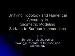
Unifying Topology and Numerical Accuracy in Geometric ModelingSurface to Surface Intersections K. H. Ko School of Mechatronics Gwangju Institute of Science and Technology
Motivations • Digital Laboratory, digital manufacturing, computer simulation, etc. • Physical mockup creation and evaluation • Time consuming and expensive • Evaluation of models with various changes is not practical. • Evaluation using virtual computer models • Allows us to evaluate the effects of small changes of the model. • Leads to an optimum design in an efficient manner.
Motivations • CAD is the key technology in virtual environment. • Geometric models are in the center of such a design and evaluation process. • However…..
Introduction • SIAM News, June, 1999 by R. Farouki • “… Although modern CAD systems have attained a certain degree of maturity, their efficiency, reliability, and compatibility with subsequent analysis tools fall far short of what was envisaged at their inception, some 25 years ago. At the heart of this problem lie some deep mathematical issues, concerned with the computation, representation and manipulation of complex geometries, …”
Motivations • The fundamental issue in geometric modeling is to create a (watertight) model which is • Topologically consistent • Numerically accurate • Intersection computation is the main process to create such a model. • But this is not easy!!!
Motivations • Why is this difficult??? • It is impossible to compute the exact intersections in general. • Intersections of bicubic tensor-product: the degree of the algebraic curve of intersection could reach up to 324!!! • Limitation of precision in floating point arithmetic. • Due to rounding operation, the mathematically exact equation may yield an approximation value.
Motivations • In general, they use a low degree curve to approximate the exact one of high degree. • However, this approach inevitably contains errors at the intersection!!!. • No rigorous consideration of topological consistency • Lack of numerical accuracy
Geometry Flaws - Examples • Gaps may be generated at intersections during model construction or trimming process. • In defining a solid, it causes a serious topological problem. • Confusion in determining the inside/outside of a solid.
Geometry Flaws - Examples • Problems in mesh generation. • In most cases, the mesh generation software assumes that a perfect model be given. • Defect detection and correction capability is not provided. • Therefore without manual corrections, we run into problems.
Geometry Flaws - Examples • Complex geometries are used in CAD models. • Flaws are detected and repaired manually. • Critical bottleneck for smooth integration of CAD and CFD analysis systems. • Generation of geometrically and topologically correct models will save time and money in product design.
Motivations(Summary) • Such problems prevent CAD systems from being more powerful tools in the design and development stage. • They are rooted in the generation of numerically and topologically inappropriate models. • Efficient computation of intersections considering topological and numerical aspects is important. Therefore…
Vision • From the practical view point, a curve which is topologically consistent and “sufficiently close” to the exact one can avoid any error due to approximation. • We can achieve a “watertight” solid model. • For this consider the topology and accuracy together and then combine them. • Objectives of this work focusing on intersection curves • Determination of an approximation curve for consistent topology. • Low degree curve approximation and error minimization.
Surface-to-Surface Intersections • In most cases, Rational Parametric Polynomial surface intersections are common. • Solution Methods • Lattice Method • Subdivision Method • Marching Method (Tracing method) • Marching Method is a popular choice.
Surface-to-Surface Intersections • Surface to Surface Intersection Problems • Formulated as a set of nonlinear ODE systems
Surface-to-Surface Intersections • Surface to Surface Intersection Problems • Transversal Intersection
Surface-to-Surface Intersections • Surface to Surface Intersection Problems • Tangential Intersection
Surface-to-Surface Intersections • Surface to Surface Intersection Problems • Tangential Intersection
Overall Picture Error Bound Exact Solution Curve Perturbation / Error Minimization against the exact solution Curve Approximation
Step 1 Step 2 Step 3 Step 4 Topological Configura-tion of Intersection Curves Curve Tracing and Error Bound Determina-tion Approxima-tion of Curves Error Minimiza-tion Vision Flow of Proposed Solution Intersection Curve Topology Geometric Model Topology
v=1 u=0,v=0 u=1 Topological Configuration of Intersection Curves • Computation of critical points • Use a robust and stable root solver. • Interval Projected Polyhedron Algorithm • Resolving the topological configuration of each curve segment in the parametric space. • Loop, branch, etc.
Curve Tracing and Error Bound Determination • Ordinary Numerical Solution Methods: Runge-Kutta, Adams-bashforth, etc. • Generally, they work fine. • But they may suffer from “straying or looping” problems. • Near singular points, the behavior of the methods may not be defined.
Curve Tracing and Error Bound Determination • Tracing intersection curves • Use the Validated ODE Solver • Phase I: Step size selection and a priori enclosure computation • Determination of a region where existence and uniqueness of the solution is validated. • Phase II: Tight enclosure computation • Given an a priori enclosure, a tight enclosure at the next step is computed minimizing the wrapping effect. • Using compute a tight enclosure
Conceptual Illustration of Validated ODE Solver. True solution curve Solution si si+1 si+2 Error bounds Parameter Curve Tracing and Error Bound Determination
Curve Tracing and Error Bound Determination • Phase I: Step size selection and a priori enclosure computation • To compute a step-size hj and an a priori enclosure such that, Ex. Constant Enclosure Method Tight Enclosure
Curve Tracing and Error Bound Determination • Phase II: Tight enclosure computation • Avoid the wrapping effect. • QR decomposition method
Results & Examples Transversal intersection of rational parametric surfaces Self intersection of a bi-cubic surface Intersection of a hyperbolic surface with a plane
Results & Examples Tangential intersections of parametric surfaces
Results & Examples Preventing Straying or Looping Adams-BashforthRunge-Kutta Result from a validated interval scheme
매핑 v 오차 범위 r1(u(s),v(s)) r2 β(s)=(u(s),v(s)) r1 u Curve Tracing and Error Bound Determination • Determination of error bound
Curve Tracing and Error Bound Determination s – t u – v Mapping of a priori enclosures in parametric space to 3D space
C(s) r2 r2(σ(s),t(s)) r1 r1(u(s),v(s)) v t u σ Curve Tracing and Error Bound Determination • Intersection Curve Representation • Ideally C(s) = r1(u(s),v(s)) = r2(σ(s),t(s))
Curve Tracing and Error Bound Determination • Intersection Curve Representation • However in practice, • r1(u*(s),v*(s)) ≠ r2(σ*(s),t*(s))
Approximation of Curves • It is almost impossible to compute the exact intersection curve. • We do not have an instance of intersection to work with by using the Validated ODE solver. • Any curve in the validated region can be considered as an intersection curve. • We need one curve!!!
Approximation of Curves Naïve Piecewise Linear Topologically Equivalent Approximation
Approximation of Curves Tubular Neighborhood by Offsets
Small neighborhood 1 intersection Approximation of Curves
C(s) r2 r2(σ(s),t(s)) r1 r1(u(s),v(s)) v t u σ Approximation of Curves • We take the center points at each step and approximate them using a cubic B-spline curve in each u-v and σ–t parametric space. • r1(u*(s),v*(s)), and r2(σ*(s),t*(s)) in 3D space • But r1 ≠ r2. • But each should be within the validated region.
Curve approximation Approximation of Curves Solution si si+1 si+2 Parameter
Error Minimization • The approximated B-spline curve is perturbed to minimize the error between two space curves r1(u*(s),v*(s)) and r2(σ*(s),t*(s)). • Curve perturbation through minimization • Given points Yk(k=1,2,…,n) and the approximated B-spline curve P(t). • Then find the control points Pi (i=1,2,…,m) which minimize the following.
C(s) r2 r2(σ(s),t(s)) r1 r1(u(s),v(s)) v t u σ Error Minimization • Adjust the curves in u-v and σ–t parametric spaces such that the error in 3D space becomes minimal. • In this case, the objective function needs to be reformulated. Error minimization
Conclusions • Compute an approximate curve which is “sufficiently close” to the exact one. • Topologically consistent • Numerically accurate. • Theoretical and practical foundation on watertight solid model creation. • Provide a smooth interface between CAD systems and downstream applications. • Mesh creation
References • Bajaj, C. L. and Xu, G., 1994, NURBS Approximation of Surface/Surface Intersection Curves, Advances in Computational Mathematics, 2, pp. 1-21. • Farouki, R. T., 1999, Closing the gap between CAD model and downstream application, SIAM News, 32 (5), pp. 1-3. • Grandine, T. A. and Klein, F. W., 1997, A new approach to the surface intersection problem, Computer Aided Geometric Design, 14, pp. 111-134. • Hoschek, J. and Lasser, D., 1993, Fundamentals of Computer Aided Geometric Design, A K Peters, Wellesley, MA. • Katz, S., and Sederberg, T. W., 1988, Genus of the intersection curve of two rational surface patches, Computer Aided Geometric Design, 5, pp. 253-258. • Lohner, R. J., 1992, Computation of guaranteed enclosures for the solutions of ordinary initial and boundary value problem, In Computational Ordinary Differential Equations, Cash J., Gladwell I., (Eds.), Clarendon Press, Oxford, pp. 425-235. • Maekawa, T., Patrikalakis, N. M., Sakkalis, T., and Yu, G., 1998, Analysis and Applications of Pipe Surfaces, Computer Aided Geometric Design. 15(5), pp. 437-458. • Mukundan, H, Ko, K. H., Maekawa, T., Sakkalis, and T., Patrikalakis, N. M., 2004, Tracing Surface Intersections with a Validated ODE System Solver, Proceedings of the 9th EG/ACM Symposium on Solid Modeling and Applications, G. Elber, N. Patrikalakis and P. Brunet, editors. pp. 249-254. Genoa, Italy, Eurographics Press. • Nedialkov, N. S., Jackson, K. R., and Corliss, G. F., 1999, Validated solutions of initial value problems for ordinary differential equations, Applied Mathematics and Computation, 105(1), pp. 21-68.
References • Patrikalakis, N. M., and Maekawa, T., 2002, Shape Interrogation for Computer Aided Design and Manufacturing, Springer, New York. • Peters, T. J., 2003, Intersecting Surfaces and Approximated Topology, ECG Workshop on applications Involving Geometric Algorithms with Curved Objects, Saarbrüken, Germany. • Sakkalis, T., 1991, The topological configuration of a real algebraic curve, Bulletin of the Australian Mathematical Society, 43, pp. 37-50. • Sederberg, T. W. 1983, Implicit and parametric curves and surfaces for computer aided geometric design, PhD Thesis, Purdue University. • Shen, G., 2000, Analysis of Boundary Representation Model Rectification, PhD Thesis, Massachusetts Institute of Technology, Cambridge, MA. • Song, X., Sederberg, T. W., Zheng, J., Farouki, R. T. and Hass, J., 2004, Linear perturbation methods for topologically consistent representations of free-form surface intersections, Computer Aided Geometric Design, 21(3), pp. 303-319. • Wang, W., Pottmann, H., Liu, Y., 2004, Fitting B-Spline Curves to Point Clouds by Squared Distance Minimization, HKU CS Technical Report TR-2004-11.