Download
1 / 48
490 likes | 579 Views
Explore various biological networks such as protein-protein interactions, regulatory networks, and metabolic networks. Learn about network hierarchies, genetic interactions, and more. Discover graph theory basics and network models like Erdos-Renyi and Watts-Strogatz.

E N D
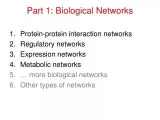
Part 1: Biological Networks • Protein-protein interaction networks • Regulatory networks • Expression networks • Metabolic networks • … more biological networks • Other types of networks
Expression networks [Qian, et al, J. Mol. Bio., 314:1053-1066]
Regulatory networks [Horak, et al, Genes & Development, 16:3017-3033]
Regulatory networks Expression networks
Interaction networks Regulatory networks Expression networks
Metabolic networks [DeRisi, Iyer, and Brown, Science, 278:680-686]
Regulatory networks Expression networks Interaction networks Metabolic networks
... more biological networks Hierarchies & DAGs [Enzyme, Bairoch; GO, Ashburner; MIPS, Mewes, Frishman]
Gene order networks Genetic interaction networks [Boone] Neural networks [Cajal] ... more biological networks
Other types of networks Disease Spread [Krebs] Electronic Circuit Food Web Internet [Burch & Cheswick] Social Network
Part 2: Graphs, Networks Graph definition Topological properties of graphs Degree of a node Clustering coefficient Characteristic path length Random networks Small World networks Scale Free networks
Graph: a pair of sets G={P,E} where P is a set of nodes, and E is a set of edges that connect 2 elements of P. • Directed, undirected graphs • Large, complex networks are ubiquitous in the world: • Genetic networks • Nervous system • Social interactions • World Wide Web
Degree of a node:the number of edges incident on the node i Degree of node i = 5
Clustering coefficient LOCAL property • The clustering coefficient of node i is the ratio of the number of edges that exist among its neighbours, over the number of edges that could exist Clustering coefficient of node i = 1/6 • The clustering coefficient for the entire network C is the average of all the
i j • The characteristic path length L of a graph is the average of the for every possible pair (i,j) Characteristic path length GLOBAL property • is the number of edges in the shortest path between vertices i and j Networks with small values of L are said to have the “small world property”
Models for networks of complex topology • Erdos-Renyi (1960) • Watts-Strogatz (1998) • Barabasi-Albert (1999)
The Erdős-Rényi [ER] model (1960) • Start with N vertices and no edges • Connect each pair of vertices with probability PER • Important result: many properties in these graphs appear quite suddenly, at a threshold value of PER(N) • If PER~c/N with c<1, then almost all vertices belong to isolated trees • Cycles of all orders appear at PER ~ 1/N
The Watts-Strogatz [WS] model (1998) • Start with a regular network with N vertices • Rewire each edge with probability p • For p=0 (Regular Networks): • high clustering coefficient • high characteristic path length • For p=1 (Random Networks): • low clustering coefficient • low characteristic path length QUESTION: What happens for intermediate values of p?
1) There is a broad interval of p for which L is small but C remains large 2) Small world networks are common :
The Barabási-Albert [BA] model (1999) Look at the distribution of degrees ER Model ER Model WS Model www actors power grid The probability of finding a highly connected node decreases exponentially with k
● two problems with the previous models: 1. N does not vary 2. the probability that two vertices are connected is uniform • GROWTH: starting with a small number of vertices m0 at every timestep add a new vertex with m ≤ m0 • PREFERENTIAL ATTACHMENT: the probability Π that a new vertex will be connected to vertex i depends on the connectivity of that vertex:
a) Connectivity distribution with N = m0+t=300000 and m0=m=1(circles), m0=m=3 (squares), and m0=m=5 (diamons) and m0=m=7 (triangles) b) P(k) for m0=m=5 and system size N=100000 (circles), N=150000 (squares) and N=200000 (diamonds) Scale Free Networks
Part 3: Machine Learning • Artificial Intelligence/Machine Learning • Definition of Learning • 3 types of learning • Supervised learning • Unsupervised learning • Reinforcement Learning • Classification problems, regression problems • Occam’s razor • Estimating generalization • Some important topics: • Naïve Bayes • Probability density estimation • Linear discriminants • Non-linear discriminants (Decision Trees, Support Vector Machines)
PROBLEM: we are given and we have to decide whether it is an a or a b Classification Problems Bayes’ Rule:minimum classification error is achieved by selecting the class with largest posterior probability
Regression Problems PROBLEM: we are only given the red points, and we would like approximate the blue curve (e.g. with polynomial functions) QUESTION: which solution should I pick? And why?
Naïve Bayes Example: given a set of features for each gene, predict whether it is essential
Bayes Rule: select the class with the highest posterior probability For a problem with two classes this becomes: if then choose class otherwise, choose class
For a two classes problem: where and are called Likelihood Ratio for feature i. Naïve Bayes approximation:
Probability density estimation • Assume a certain probabilistic model for each class • Learn the parameters for each model (EM algorithm)
Linear discriminants • assume a specific functional form for the discriminant function • learn its parameters
Decision Trees (C4.5, CART) • ISSUES: • how to choose the “best” attribute • how to prune the tree Trees can be converted into rules !
Part 4: Networks Predictions • Naïve Bayes for inferring Protein-Protein Interactions
Feature 1, e.g. co-expression Feature 2, e.g. same function Gold-standard + Gold-standard – The data Gold-Standards Network [Jansen, Yu, et al., Science; Yu, et al., Genome Res.]
Feature 1, e.g. co-expression Feature 2, e.g. same function Gold-standard + Gold-standard – Likelihood Ratio for Feature i: Gold-Standards Network
Feature 1, e.g. co-expression Feature 2, e.g. same function Gold-standard + Gold-standard – Likelihood Ratio for Feature i: Gold-Standards Network L1 = (4/4)/(3/6) =2
Feature 1, e.g. co-expression Feature 2, e.g. same function Gold-standard + Gold-standard – Likelihood Ratio for Feature i: Gold-Standards Network L1 = (4/4)/(3/6) =2
Feature 1, e.g. co-expression Feature 2, e.g. same function Gold-standard + Gold-standard – Likelihood Ratio for Feature i: Gold-Standards Network L1 = (4/4)/(3/6) =2
Feature 1, e.g. co-expression Feature 2, e.g. same function Gold-standard + Gold-standard – Likelihood Ratio for Feature i: Gold-Standards Network L1 = (4/4)/(3/6) =2
Feature 1, e.g. co-expression Feature 2, e.g. same function Gold-standard + Gold-standard – Likelihood Ratio for Feature i: Gold-Standards Network L1 = (4/4)/(3/6) =2
Feature 1, e.g. co-expression Feature 2, e.g. same function Gold-standard + Gold-standard – Likelihood Ratio for Feature i: Gold-Standards Network L1 = (4/4)/(3/6) =2 L2 = (3/4)/(3/6) =1.5 For each protein pair: LR = L1 L2 log(LR) = log(L1) + log(L2)
Feature 1, e.g. co-expression Feature 2, e.g. same function Gold-standard + Gold-standard – Likelihood Ratio for Feature i: Gold-Standards Network L1 = (4/4)/(3/6) =2 L2 = (3/4)/(3/6) =1.5 For each protein pair: LR = L1 L2 log(LR) = log(L1) + log(L2)
Individual features are weak predictors, • LR ~ 10; • Bayesian integration is much more powerful, • LRcutoff = 600 ~9000 interactions