Download
1 / 32
320 likes | 347 Views
This study presents numerical simulation results of concentrated non-Brownian suspensions in viscous fluids from a granular point of view. The simulation considers quasistatic response, steady shear flow, hydrodynamic forces, and the role of contacts. Results provide insights into the critical state, friction coefficient, and behavior under large strain.

E N D
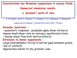
Concentrated non-Brownian suspensions in viscous fluids. Numerical simulation results, a “granular” point of view J.-N. Roux,with F. Chevoir, F. Lahmar, P.-E. Peyneau, S. Khamseh Laboratoire Navier, Université Paris-Est, France Granular materials : • quasistatic response : gradually apply shear stress or impose small shear rate on isotropic equilibrated state • steady shear flow with inertial effects Extension to dense suspensions : Large hydrodynamic forces in narrow gaps between grains, role of contacts Approaches similar to dry granular case
Granular materials : initial density and critical state Monodisperse sphere assembly, friction coefficient = 0.3 Several samples with 4000 beads, prepared at different solid fraction Triaxial test Similar response in simple shear test ! Under large strain, critical state independent of initial state, characterized by a ‘’flow structure’’ (density + nb of contacts, anisotropy…)
Critical state of dry granular materials, 2D and3D results Compilation of simulation literature, in Lemaître, Roux & Chevoir, Rheologica Acta 2009 c and c do not depend on contact stiffness if large enough Internal friction coefficient (actually somewhat different between shear tests and other load directions, e.g. triaxial, see e.g., Peyneau & Roux, PRE 2008) Critical solid fraction c = RCP for = 0
What we know from simulations of dry grains (I) Quasistatic rheology : • interest of critical state concept (flow structure) c minimum solid fraction in flow • Friction coefficient in contacts determines c and *c. Small rolling frictionalso quite influential • using contact law and applied pressure P, define stiffness number (suchthat deflection is prop. to-1), assess approach to rigid grain limit Inertial flows : • Study shear flow under controlled normal stress rather than fixed density : non-singular quasistatic limit • use internal friction * as an alternative to viscosity
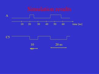
Simulation of steady uniform shear flow Normal stress is imposed Fixed shear strain rate
What we know from studies on dry grains (II) : Inertial number and constitutive relations Material state in shear flow ruled by one dimensionless parameter, the inertial number Monodisperse spheres, no intergranular friction (Peyneau & Roux, Phys Rev E 2008) RCP Generalization of critical state to I-dependent states with inertial effects Useful constitutive law, applied to different geometries (Pouliquen, Jop, Forterre…)
Steady shear flow of dry, frictionless beads at low I number : normal stress-controlled vs. volume controlled (P.-E. Peyneau) Same behavior, very large stress fluctuations if is imposed (4000 grains) Ratio 12/22 = * expresses material rheology
Simulations of dense suspensions • in simulation literature : nothing for > 0.6 (spheres), ad-hoc repulsive forces used to push grains apart, very few published results with N >1000… • sharp contrast with simulations of dry grains! • lubrication singularities believed to lead to some dynamic jamming phenomenon below RCP (related to possible origin of shear thickening) Ball and Melrose, 1995-2004: no steady state (!?) • Here : control normal stress rather than density, control lubrication cutoff and contact interaction stiffness Experiments on dense suspensions • Attention paid to possible density inhomogeneities local measurements • Boyer et al. control of particle pressure !
Simulation of very dense suspensions • Simplified modeling approach, fluid limited to near-neighbor gaps and pairwise lubrication interactions (cf. Melrose & Ball) • Lubrication singularity cut off at short distance. Contact forces (or short–range repulsion due to polymer layer) • Stokes régime : contact, external and viscous forces balance Questions Divergence of at < RCP ? Sensitivity to repulsive forces ? To alone ? Effective viscosity, non-Newtonian effects, normal stresses…
Lubrication and hydrodynamic resistance matrix Normal hydrodynamic force : For 2 spheres of radius R, with perfect lubrication : dominant forces transmitted by a network of ‘quasi-contacts’ No contact within finite time ! Cut-off for narrow interstices h<hmin (asperities), contact becomes possible Without cutoff: both physically irrelevant and computationally untractable
Choice of systems and parameters D systems of identical spheres, diameter a : • tobeads • hmax/a = 0.1 or 0.3 • hmin/a = 10-4 ; = 105 • Vi from 0.1 down to 5.10-4 • = 0 in solid contacts • + alternative systems with repulsive forces, no lubrication cutoff D systems of polydisperse disks, diameter d, • disks • 3D lubrication • hmax/a = 0.5 • hmin/a = 10-4 or 10-2; = 104 • Vi down to 10-4 or10-6 • = 0.3 in solid contacts
Model, computation method • assemble hydrodynamic resistance matrix (similar to stiffness matrix in elastic contact network) • non-singular tangential coefficient • add up ‘ordinary’ contact forces (elasticity + friction) to viscous hydrodynamic ones when grains touch (simple approximation) with and Fc depend on grain positions Solve
Some technical aspects about simulations Lees-Edwards boundary conditions + variable height,ensuring constant yy Measurements in steady state : • Check for stationarity of measurements • Obtain error bar from ‘blocking’ technique • Request long enough stationary intervals Regression of fluctuations Constant volume and/or constant shear stress conditions should produce same system state in large N limit N -1/2 N -1/2
Choice of time step, integration t such that matrix and r.h.s. do not change `too much’… Euler (explicit) : (error ~t2) ‘Trapezoidal’ rule : (error ~ t3)
A crucial test on the numerical integration of equations of motion Relative difference between variation of h and integration of normal relative velocity in various interstices, 2 different numerical schemes : Euler (dotted lines), trapezoidal (continuous lines) Keep it below 0.05 !
Controlparameter for dense suspensions : viscous number Vi Plays analogous role to inertia parameter defined for dry grains Vi = (decay time of h(t) in compressed layer within gap) / (shear time) I = (acceleration time) / (shear time) Acceleration (inertial) time replaced by a squeezing time in viscous layer Cassar, Nicolas, Pouliquen, Phys. of Fluids 2005 (similar Vi, with drainage time)
Steady shear flow of lubricated beads at low Vi number : normal stress-controlled vs. volume controlled Vi = 10-3 Same behavior, large stress fluctuations if is imposed (1372 grains). Ratio 12/22 = * expresses material rheology
3D results : *and as functions of Vi identical spherical grains Vi Vi = 0 : difficultcase ! Approach to * = 0.1, =0.64 …
Back to more traditional (constant ) approach Effective viscosity From and one gets: (not satisfiedin our case !) if Exponent : 2.5 to 3 ? Shear rate effects ? In rigid grain limit replace 4th argument by zero. No influenceof on effective viscosity
Effective viscosity, as a fonction of solid fraction (hc = hmax)
Ordered structure polydispersity < 20% Influence of repulsive force Adsorbed polymer layer, short-range repulsion, as Polymer layer thickness lb = 0.01 or 0.001 (open/filled symbols ) Force F0 ratio F0/a2P (0.1, 1, 10) = (diamond, square, circle) (Fredrickson & Pincus, 1991) Shear-thinning within studied parameter range Vic ~ 3.10-2 Pair correlations in plane yz
Shear thinning with repulsive forces Shear thinning due to change in reduced shear rate Results correspond to varying from 5.10-5 to 10-1 No shear thinning for smaller lb
Network of repulsive forces carry all shear stress as Vi decreases Vi Other ‘granular’ features: force distribution, coordination number…
Viscosity of random, isotropic suspensions • Assume ideal hard sphere particle distribution at given • Measure instantaneous shear viscosity Comparison with Stokesian Dynamics results: encouraging agreement at large densities, although treatment of subdominant terms not entirely innocuous
3D frictionless spherical beads : • Analogy with dry granular flow • Difficulty to approach quasistatic limit • No singularity below RCP density, a steady-state can be reached • Importance of non-hydrodynamic interactions • Purely hydrodynamic model approached with stiff interactions • Effects of additional forces: 2-parameter space to be explored 2D disk model Easier system, introduction of tangential forces, friction, faster approach to quasistatic limit Show coincidence of quasistatic limits for dry grains and dense suspension
2D results : internal friction coefficient versus Vi (analogous to function of I in dry inertialcase) Viscous Dry, inertial Viscous case hmin/a = 10-2 and hmin/a = 10-4 , =0,3 Dry inertial case (right) : =0.3 and =0 Coincidence I=0 / Vi=0
2D results :solid fraction versus Vi (in paste) (analogous to function of I in dry inertial case) Dry, inertial Viscous Viscous case hmin/a = 10-2 and hmin/a = 10-4 (896 grains), =0.3 Dry inertial case(right) : =0.3 and =0 Coincidence I=0 /Vi =0
Constitutive laws : dry grains (2D) = 0 or 0.3 Constitutive laws, granular suspensions (2D), = 0.3 Same constant terms (quasistatic limit), different power laws
Effective viscosity, as a function of solid fraction • Divergence of effective viscosity as critical solid fraction c is approached • (once again) no accurate determination of exponent (2 ? 2.5 ?) • Little influence of roughness length scale
Importance of direct contact interactions Pressure due to solid contact forces / total pressure (Case hmin/a = 10-2)
Some conclusions on dense suspensions • interesting to study dense suspensions under controlled normal stress • importance of contact interactions : solid friction, asperities…) Contact or static forces dominate at low Vi • relevance of critical stateas initially introduced in soil mechanics. Viscosity diverges as approaches c • With =0 in contacts, no jamming or viscosity divergence or any specific singularity below RCP, except in small systems • If is large enough, * independent of with elastic (-frictional) beads (but… Re ? Brownian effects ?) • introduction of repulsive interaction with force scale shear-thinning (or thickening)
Perspectives Improve performance of numerical methods Continuum fluid ! (Keep separate treatment of lubrication singularities ?) bridge the gap between real (and difficult) hydrodynamic calculations and ‘conceptual models’