Download

1 / 39
390 likes | 588 Views
Software abstractions for many-core software engineering. Paul H J Kelly Group Leader, Software Performance Optimisation Department of Computing Imperial College London Joint work with : David Ham, Gerard Gorman, Florian Rathgeber (Imperial ESE/Grantham Inst for Climate Change Res)

E N D
Software abstractions for many-core software engineering Paul H J Kelly Group Leader, Software Performance Optimisation Department of Computing Imperial College London Joint work with : David Ham, Gerard Gorman, Florian Rathgeber (Imperial ESE/Grantham Inst for Climate Change Res) Mike Giles, GihanMudalige (Mathematical Inst, Oxford) Adam Betts, Carlo Bertolli, Graham Markall, Tiziano Santoro, George Rokos (Software Perf Opt Group, Imperial) Spencer Sherwin (Aeronautics, Imperial), Chris Cantwell (Cardio-mathematics group, Mathematics, Imperial)
What we are doing…. Quantum chemistry Vision & 3D3D scene understanding Rolls-Royce HYDRA turbomachinery CFD LAMMPS – granular flow FENiCS finite-element PDE generator Fluidity and the Imperial College Ocean Model (ICOM) Multicore Form Compiler Moving meshes Finite-volume CFD Particle problems – molecular dynamics Finite-element assembly Mesh adaptation Mixed meshes P-adaptivity Pair_gen for LAMMPS OP2: parallel loops over unstructured meshes OP2.1: extended with dynamic meshes OP2.2: extended with sparse matrices OP2.3: with fully-abstract graphs OP2.4: mixed and piecewise structured meshes Fortran & C/C++ OP2 compiler CUDA/OpenCL OpenMP MPI SSE/AVX FPGAs ? • Roadmap: applications drive DSLs, delivering performance portability
The message • Three slogans Three stories • Generative, instead of transformative optimisation • Domain-specific active library examples • Get the abstraction right, to isolate numerical methods from mapping to hardware • General framework: access-execute descriptors • The value of generative and DSL techniques • Build vertically, learn horizontally
Easy parallelism – tricky engineering • Parallelism breaks abstractions: • Whether code should run in parallel depends on context • How data and computation should be distributed across the machine depends on context • “Best-effort”, opportunistic parallelisation is almost useless: • Robust software must robustly, predictably, exploit large-scale parallelism How can we build robustly-efficient multicore software While maintaining the abstractions that keep code clean, reusable and of long-term value? It’s a software engineering problem
Active libraries and DSLs Visual effects • Domain-specific languages... • Embedded DSLs • Active libraries • Libraries that come with a mechanism to deliver library-specific optimisations • Domain-specific “active” library encapsulates specialist performance expertise • Each new platform requires new performance tuning effort • So domain-specialists will be doing the performance tuning • Our challenge is to support them Finite element Linear algebra Game physics Finite difference Applications Active library Exotic hardware Multicore GPU FPGA Quantum?
Program Dependence Parallelisation Synthesis Tiling ..... Analysis Storage layout Shape Instruction selection/scheduling Dependence Register allocation Class-hierarchy Points-to Syntax • Classical compilers have two halves
Program Dependence Parallelisation Synthesis Tiling ..... Analysis Storage layout Shape Instruction selection/scheduling Dependence Register allocation Class-hierarchy Points-to Syntax • The right domain-specific language or active library can give us a free ride
Program Dependence Parallelisation Synthesis Tiling ..... Analysis Storage layout Shape Instruction selection/scheduling Dependence Register allocation http://www.nikkiemcdade.com/subFiles/2DExamples.html http://www.ginz.com/new_zealand/ski_new_zealand_wanaka_cadrona Class-hierarchy Points-to Syntax • It turns out that analysis is not always the interesting part....
C,C++, C#, Java, Fortran Capture dependence and communication in programs over richer data structures Specify application requirements, leaving implementation to select radically-different solution approaches Code motion optimisations Vectorisation and parallelisation of affine loops over arrays
Encapsulating and delivering domain expertise • Domain-specific languages & active libraries • Raise the level of abstraction • Capture a domain of variability • Encapsulate reuse of a body of code generation expertise/techniques • Enable us to capture design space • To match implementation choice to application context: • Target hardware • Problem instance • This talk illustrates these ideas with some of our recent/current projects Application-domain context Unifying representation Target hardware context
OP2 – a decoupled access-execute active library for unstructured mesh computations floatu_sum, u_max, beta = 1.0f; for( int iter = 0; iter < NITER; iter++ ) {op_par_loop( res, edges, op_arg_dat( p_A, 0, NULL, OP_READ ), op_arg_dat( p_u, 0, &pedge2, OP_READ ), op_arg_dat( p_du, 0, &pedge1, OP_INC ), op_arg_gbl( &beta, OP_READ ) ); u_sum= 0.0f; u_max = 0.0f; op_par_loop( update, nodes, op_arg_dat( p_r, 0, NULL, OP_READ ), op_arg_dat( p_du, 0, NULL, OP_RW ), op_arg_dat( p_u, 0, NULL, OP_INC ), op_arg_gbl( &u_sum, OP_INC ), op_arg_gbl( &u_max, OP_MAX ) ); } // declare sets, maps, and datasets op_setnodes= op_decl_set( nnodes ); op_setedges= op_decl_set( nedges ); op_mappedge1 = op_decl_map(edges, nodes, 1, mapData1 ); op_mappedge2 = op_decl_map(edges, nodes, 1, mapData2 ); op_datp_A = op_decl_dat(edges, 1, A ); op_datp_r = op_decl_dat(nodes, 1, r ); op_datp_u = op_decl_dat(nodes, 1, u ); op_datp_du = op_decl_dat(nodes, 1, du ); // global variables and constants declarations float alpha[2] = { 1.0f, 1.0f }; op_decl_const( 2, alpha ); Example – Jacobi solver
OP2- Data model // declare sets, maps, and datasets op_setnodes= op_decl_set( nnodes ); op_setedges= op_decl_set( nedges ); op_mappedge1 = op_decl_map(edges, nodes, 1, mapData1 ); op_mappedge2 = op_decl_map(edges, nodes, 1, mapData2 ); op_datp_A = op_decl_dat(edges, 1, A ); op_datp_r = op_decl_dat(nodes, 1, r ); op_datp_u = op_decl_dat(nodes, 1, u ); op_datp_du = op_decl_dat(nodes, 1, du ); // global variables and constants declarations float alpha[2] = { 1.0f, 1.0f }; op_decl_const( 2, alpha ); A Pedge1 Pedge2 A Pedge1 Pedge2 A Pedge1 Pedge2 A Pedge1 Pedge2 A Pedge1 Pedge2 r u Du r u Du r u Du r u Du r u Du r u Du OP2’s key data structure is a set A set may contain pointers that map into another set Eg each edge points to two vertices
OP2 – a decoupled access-execute active library for unstructured mesh computations floatu_sum, u_max, beta = 1.0f; for( int iter = 0; iter < NITER; iter++ ) {op_par_loop_4 ( res, edges, op_arg_dat( p_A, 0, NULL, OP_READ ), op_arg_dat( p_u, 0, &pedge2, OP_READ ), op_arg_dat( p_du, 0, &pedge1, OP_INC ), op_arg_gbl( &beta, OP_READ ) ); u_sum= 0.0f; u_max = 0.0f; op_par_loop_5 ( update, nodes, op_arg_dat ( p_r, 0, NULL, OP_READ ), op_arg_dat ( p_du, 0, NULL, OP_RW ), op_arg_dat( p_u, 0, NULL, OP_INC ), op_arg_gbl( &u_sum, OP_INC ), op_arg_gbl( &u_max, OP_MAX ) ); } • Each parallel loop precisely characterises the data that will be accessed by each iteration • This allows staging into scratchpad memory • And gives us precise dependence information • In this example, the “res” kernel visits each edge • reads edge data, A • Reads beta (a global), • Reads u belonging to the vertex pointed to by “edge2” • Increments du belonging to the vertex pointed to by “edge1” Example – Jacobi solver
OP2 – parallel loops inlinevoidres(constfloatA[1], constfloatu[1], floatdu[1], constfloatbeta[1]) { du[0] += beta[0]*A[0]*u[0]; } floatu_sum, u_max, beta = 1.0f; for( int iter = 0; iter < NITER; iter++ ) {op_par_loop_4 ( res, edges, op_arg_dat( p_A, 0, NULL, OP_READ ), op_arg_dat( p_u, 0, &pedge2, OP_READ ), op_arg_dat( p_du, 0, &pedge1, OP_INC ), op_arg_gbl( &beta, OP_READ ) ); u_sum= 0.0f; u_max = 0.0f; op_par_loop_5 ( update, nodes, op_arg_dat( p_r, 0, NULL, OP_READ ), op_arg_dat( p_du, 0, NULL, OP_RW ), op_arg_dat( p_u, 0, NULL, OP_INC ), op_arg_gbl( &u_sum, OP_INC ), op_arg_gbl( &u_max, OP_MAX ) ); } • Each parallel loop precisely characterises the data that will be accessed by each iteration • This allows staging into scratchpad memory • And gives us precise dependence information • In this example, the “res” kernel visits each edge • reads edge data, A • Reads beta (a global), • Reads u belonging to the vertex pointed to by “edge2” • Increments du belonging to the vertex pointed to by “edge1” inlinevoidupdate(constfloatr[1],floatdu[1], floatu[1], floatu_sum[1], floatu_max[1]) { u[0] += du[0] + alpha * r[0]; du[0] = 0.0f; u_sum[0] += u[0]*u[0]; u_max[0] = MAX(u_max[0],u[0]); } Example – Jacobi solver
Two key optimisations: • Partitioning • Colouring Edges Cross-partition edges Vertices
Two key optimisations: • Partitioning • Colouring • Elements of the edge set are coloured to avoid races due to concurrent updates to shared nodes Edges Cross-partition edges Vertices
Two key optimisations: • Partitioning • Colouring • At two levels Edges Cross-partition edges Vertices
OP2 - performance • Example: non-linear 2D inviscid unstructured airfoil code, double precision (compute-light, data-heavy) • Three backends: OpenMP, CUDA, MPI (OpenCL coming) • For tough, unstructured problems like this GPUs can win, but you have to work at it • X86 also benefits from tiling; we are looking at how to enhance SSE/AVX exploitation
Combining MPI, OpenMP and CUDA non-linear 2D inviscidairfoilcode 26M-edge unstructured mesh 1000 iterations Analytical model validated on up to 120 Westmere X5650 cores and 1920 HECToR (Cray XE6 Magny-Cours) cores Unmodified C++ OP2 source code exploits inter-node parallelism using MPI, and intra-node parallelism using OpenMP and CUDA (Mudalige et al, PER2012)
A higher-level DSL • Solving: • Weak form: (Ignoring boundaries) Psi = state.scalar_fields(“psi”) v=TestFunction(Psi) u=TrialFunction(Psi) f=Function(Psi, “sin(x[0])+cos(x[1])”) A=dot(grad(v),grad(u))*dx RHS=v*f*dx Solve(Psi,A,RHS) UFL – Unified Form Language (FEniCSproject, http://fenicsproject.org/):A domain-specific language for generating finite element discretisations of variational forms Specify application requirements, leaving implementation to select radically-different solution approaches
The FE Method: computation overview • Key data structures: Mesh, dense local assembly matrices, sparse global system matrix, and RHS vector i do element = 1,N assemble(element) end do j k i j k i i j j Ax = b k k
Global Assembly – GPU Issues Parallelising the global assembly leads to performance/correctness issues: • Bisection search: uncoalesced accesses, warp divergence • Contending writes: atomic operations, colouring • In some circumstances we can avoid building the global system matrix altogether • Goal: get the UFL compiler to pick the best option Local matrix for element 1 Global matrix • Set 1 • Set 2 Local matrix for element 2
The Local Matrix Approach Why do we assemble M? In the Local Matrix Approach we recompute this, instead of storing it: b is explicitly required Assemble it with an SpMV: We need to solve where
Test Problem Implementation Advection-Diffusion Equation: Solved using a split scheme: Advection: Explicit RK4 Diffusion: Implicit theta scheme GPU code: expanded data layouts, with Addto or LMA CPU baseline code: indirect data layouts, with Addto [Vos et al., 2010](Implemented within Fluidity) Double Precision arithmetic Simulation run for 200 timesteps Simplified CFD test problem
Test Platforms Nvidia 280GTX: 240 stream processors: 30 multiprocessors with 8 SMs each 1GB RAM (4GB available in Tesla C1060) NVidia 480GTX: 480 stream processors: 15 multiprocessors with 32 SMs each 1.5GB RAM (3GB available in Tesla C2050, 6GB in Tesla C2060) AMD Radeon 5870: 1600 stream processors: 20 multiprocessors with 16 5-wide SIMD units 1GB RAM (768MB max usable) Intel Xeon E5620: 4 cores 12GB RAM Software: Ubuntu 10.04 Intel Compiler 10.1 for Fortran (-O3 flag) NVIDIA CUDA SDK 3.1 for CUDA ATI Stream SDK 2.2 for OpenCL Linear Solver: CPU: PETSc [Balay et al., 2010] CUDA Conjugate Gradient Solver [Markall & Kelly, 2009], ported to OpenCL
Fermi Execution times On the 480GTX (“Fermi”) GPU, local assembly is more than 10% slower than the addto algorithm (whether using atomics or with colouring to avoid concurrent updates) • Advection-Diffusion Equation: • Solved using a split scheme: • Advection: Explicit RK4 • Diffusion: Implicit theta scheme • GPU code: expanded data layouts, with Addto or LMA • CPU baseline code: indirect data layouts, with Addto [Vos et al., 2010](Implemented within Fluidity) • Double Precision arithmetic • Simulation run for 200 timesteps
Intel 4-core E5620 (Westmere EP) On the quad-core Intel Westmere EP system, the local matrix approach is slower. Using Intel’s compiler, the baseline code (using addtos and without data expansion) is faster still • Advection-Diffusion Equation: • Solved using a split scheme: • Advection: Explicit RK4 • Diffusion: Implicit theta scheme • GPU code: expanded data layouts, with Addto or LMA • CPU baseline code: indirect data layouts, with Addto [Vos et al., 2010](Implemented within Fluidity) • Double Precision arithmetic • Simulation run for 200 timesteps
Throughput compared to CPU Implementation Throughput of best GPU implementations relative to CPU (quad-core Westmere E5620) AMD 5870 and GTX480 kernel times very similar; older AMD drivers incurred overheads
Summary of results The Local Matrix Approach is fastest on GPUs Global assembly with colouring is fastest on CPUs Expanded data layouts allow coalescing and higher performance on GPUs Accessing nodal data through indirection is better on CPU due to cache, lower memory bandwidth, and arithmetic throughput
Mapping the design space – h/p • The balance between local- vs global-assembly depends on other factors • Eg tetrahedral vs hexahedral • Eg higher-order elements • Local vs Global assembly is not the only interesting option Relative execution time on CPU (dual quad Core2) Helmholtz problem with Hex elements With increasing order Execution time normalised wrt local element approach (Cantwell et al)
Mapping the design space – h/p • Contrast: with tetrahedral elements • Local is faster than global only for much higher-order • Sum factorisation never wins Relative execution time on CPU (dual quad Core2) Helmholtz problem with Tet elements With increasing order Execution time normalised wrt local assembly (Cantwell et al, provisional results under review)
End-to-end accuracy drives algorithm selection Helmholtz problem using tetrahedral elements What is the best combination of h and p? Depends on the solution accuracy required Which, in turn determines whether to choose local vs global assembly Optimum discretisation for 10% accuracy h Optimum discretisation for 0.1% accuracy Blue dotted lines show runtime of optimal strategy; Red solid lines show L2 error
A roadmap: taking a vertical view General framework AEcute: Kernels, iteration spaces, and access descriptors
Conclusions and Further Work From these experiments: Algorithm choice makes a big difference in performance The best choice varies with the target hardware The best choice also varies with problem characteristics and accuracy objectives We need to automate code generation So we can navigate the design space freely And pick the best implementation strategy for each context Application-domain context Unifying representation Target hardware context
Having your cake and eating it • If we get this right: • Higher performance than you can reasonably achieve by hand • the DSL delivers reuse of expert techniques • Implements extremely aggressive optimisations • Performance portability • Isolate long-term value embodied in higher levels of the software from the optimisations needed for each platform • Raised level of abstraction • Promoting new levels of sophistication • Enabling flexibility • Domain-level correctness C/C++/Fortran Ease of use DSL Reusable generator CUDA VHDL Performance
Where this is going • For OP2: • For aeroengineturbomachinery CFD, funded by Rolls Royce and the TSB (the SILOET programme) • In progress: • For Fluidity, and thus into the Imperial College Ocean Model • Feasibility studies in progress: UK Met Office (“Gung Ho” project), Deutsche Wetterdienst ICON model, Nektar++ • For UFL and our Multicore Form Compiler • For Fluidity, supporting automatic generation of adjoint models • Beyond: • Similar DSL ideas for the ONETEP quantum chemistry code • Similar DSL ideas for 3D scene understanding
Acknowledgements • Thanks to Lee Howes, Ben Gaster and Dongping Zhang at AMD • Partly funded by • NERC Doctoral Training Grant (NE/G523512/1) • EPSRC “MAPDES” project (EP/I00677X/1) • EPSRC “PSL” project (EP/I006761/1) • Rolls Royce and the TSB through the SILOET programme • AMD, Codeplay, Maxeler Technologies
Example application: • Imperial College Ocean Model • Dynamically adapting mesh • Focuses computational effort to resolve complex flow • Based on Imperial’s FLUIDITY software for adaptive-mesh fluid dynamics Greenland Iceland North Atlantic Gerard J. Gorman, Applied Modelling and Computation Group, http://amcg.ese.ic.ac.uk/ Test problem: thermohaline circulation - Gulf Stream, Denmark Strait Overflow Water
Unoptimised computational simulation workflow Computational model Observations Predictions Predictive Modelling Framework Mapping onto current and future hardware Automatic maintenance of adjoint model Software abstraction layer Data assimilation Optimised design Design of experiments hrp mesh adaptivity Scale-dependent parameterisation Reduced order modelling Uncertainty quantification Sensitivity analysis Risk assessment New capabilities in modelling environmental and industrial flows Refined Computational model Refined Observations Enhanced Predictions Computational simulation workflow optimised for predictive efficiency