Download
1 / 25
250 likes | 466 Views
Computational Biology, Part 16 Biochemical Kinetics II. Robert F. Murphy Copyright 1996, 1999-2009. All rights reserved. General form of ordinary differential equations.

E N D
Computational Biology, Part 16Biochemical Kinetics II Robert F. Murphy Copyright 1996, 1999-2009. All rights reserved.
General form of ordinary differential equations • For a set of n unknown functions yi (for i=1 to n) we are given a set of n functions fi that specify the derivatives of each yi with respect to some independent variable x
Euler’s method • The simplest numerical integration method is Euler’s method. It simply converts each differential to a difference • and then calculates the value of yi by multiplying the right hand side of each differential equation by the step size x
Euler’s method • We can rewrite this as a recursion formula that allows us to calculate values of the functions yi at a series of x values. We introduce a second subscript j to indicate which x value we refer to (note that yi,jnow refers to a value not a function).
Euler’s method • Note the asymmetry of this method: the derivative (fi ) that is used to span the x is calculated only for the x value at the beginning of the interval. In regions where fi is increasing with x, this leads to underestimation of y, and, in regions where fi is decreasing with x, to overestimation of y.
Euler’s method • Consider dy/dx=6x+2. The analytical solution is y=3x2+2x. • The graph shows the Euler’s method approximation for y and the analytical solution for y (along with dy/dx). Note how the approximation always underestimates y since dy/dx is increasing
Midpoint method • A better estimate would come from evaluating the fi at the midpoint of the x interval. The problem: we know x at the midpoint but we don’t know the yi at the midpoint (yet). The solution is to use Euler’s method to estimate y and then re-estimate y using the derivatives evaluated halfway along the line segment encompassing the original y.
Midpoint method (2nd order Runge-Kutte) • This is called the midpoint method or the second-order Runge-Kutte method.
Midpoint method (2nd order Runge-Kutte) • Again consider dy/dx=6x+2. • The graph shows the midpoint approximation for y and the analytical solution for y (along with dy/dx at x and x+0.5). Note that the approximation and the analytical solution are identical in this case.
Midpoint method (2nd order Runge-Kutte) • Now consider dy/dx=3y. The analytical solution is y=e3x. • The graph shows the Euler, Midpoint and analytical solutions (along with derivatives). Note that the midpoint method is better than Euler’s method but it does not give results identical to the analytical solution since dy/dx now depends on y.
Fourth-order Runge-Kutta • The midpoint method can be extended by considering other intermediate estimates. The most frequently used variation is the fourth-order Runge-Kutta method which considers one estimate at the initial point, two estimates at the midpoint, and one estimate at a trial endpoint.
Fourth-order Runge-Kutta • Here are the formulas.
Interactive demonstration • (Modify enzyme kinetics model to incorporate midpoint method)
Solving a single differential equation using Maple • (Define the differential equation dy/dx=6x+2 using the diff operator, assigning the equation to the name deq1) • (Integrate analytically using dsolve) • (Integrate using boundary condition y(0)=5) • (Integrate using boundary condition y(0)=a) • (Integrate dy/dx=bx+c analytically) • (Integrate using boundary condition y(0)=a)
Solving a single differential equation using Maple • (Define values for constants a,b,c) • (Substitute for constants using subs) • (Use subs to convert the solution that is in the form of an equation (y(x)=...) to a functional form for plotting) • (Plot the function using plot)
Solving a set of differential equations numerically using Maple • (Define the differential equations for the enzyme catalyzed reaction discussed in Part 15)
Solving a set of differential equations numerically using Maple • (Plot the solutions using odeplot) • (Plot the phase planes using odeplot)
Other systems for exploration • The following slides describe two additional biochemical systems that can be modeled by simple modifications of the model already developed.
Biochemical System 2 • Reversible catalysis.
Biochemical System 3 • Catalytic byproduct.