Overview of Query Optimization Techniques in Relational Databases
130 likes | 256 Views
This lecture discusses the principles of query optimization in relational databases, specifically focusing on the System R approach. It outlines how different query plans are selected and evaluated, with an emphasis on the cost estimation of operations. The presentation highlights important concepts such as left-deep plans, the significance of statistics from system catalogs, and the impact of input cardinalities on optimization. Concrete examples are provided, including analysis of nested queries and plans that leverage indexes for efficient execution.

Overview of Query Optimization Techniques in Relational Databases
E N D
Presentation Transcript
Relational Query Optimization Module 5, Lecture 2
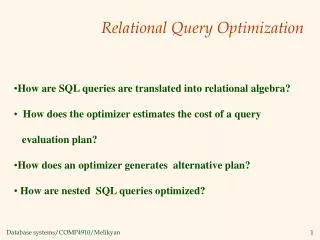
Overview of Query Optimization • Plan:Tree of R.A. ops, with choice of alg for each op. • Each operator typically implemented using a `pull’ interface: when an operator is `pulled’ for the next output tuples, it `pulls’ on its inputs and computes them. • Two main issues: • For a given query, what plans are considered? • Algorithm to search plan space for cheapest (estimated) plan. • How is the cost of a plan estimated? • Ideally: Want to find best plan. Practically: Avoid worst plans! • We will study the System R approach.
Highlights of System R Optimizer • Impact: • Most widely usedcurrently; works well for < 10 joins. • Cost estimation: Approximate art at best. • Statistics, maintained in system catalogs, used to estimate cost of operations and result sizes. • Considers combination of CPU and I/O costs. • Plan Space: Too large, must be pruned. • Only the space of left-deep plans is considered. • Left-deep plans allow output of each operator to be pipelinedinto the next operator without storing it in a temporary relation. • Cartesian products avoided.
Schema for Examples Sailors (sid: integer, sname: string, rating: integer, age: real) Reserves (sid: integer, bid: integer, day: dates, rname: string) • Similar to old schema; rname added for variations. • Reserves: • Each tuple is 40 bytes long, 100 tuples per page, 1000 pages. • Sailors: • Each tuple is 50 bytes long, 80 tuples per page, 500 pages.
sname rating > 5 bid=100 sid=sid Sailors Reserves (On-the-fly) sname (On-the-fly) rating > 5 bid=100 (Simple Nested Loops) sid=sid Sailors Reserves RA Tree: Motivating Example SELECT S.sname FROM Reserves R, Sailors S WHERE R.sid=S.sid AND R.bid=100 AND S.rating>5 • Cost: 500+500*1000 I/Os • By no means the worst plan! • Misses several opportunities: selections could have been `pushed’ earlier, no use is made of any available indexes, etc. • Goal of optimization: To find more efficient plans that compute the same answer. Plan:
(On-the-fly) sname (Sort-Merge Join) sid=sid (Scan; (Scan; write to write to rating > 5 bid=100 temp T2) temp T1) Reserves Sailors Alternative Plans 1 (No Indexes) • Main difference: push selects. • With 5 buffers, cost of plan: • Scan Reserves (1000) + write temp T1 (10 pages, if we have 100 boats, uniform distribution). • Scan Sailors (500) + write temp T2 (250 pages, if we have 10 ratings). • Sort T1 (2*2*10), sort T2 (2*3*250), merge (10+250) • Total: 3560 page I/Os. • If we used BNL join, join cost = 10+4*250, total cost = 2770. • If we `push’ projections, T1 has only sid, T2 only sid and sname: • T1 fits in 3 pages, cost of BNL drops to under 250 pages, total < 2000.
(On-the-fly) sname Alternative Plans 2With Indexes (On-the-fly) rating > 5 (Index Nested Loops, with pipelining ) sid=sid • With clustered index on bid of Reserves, we get 100,000/100 = 1000 tuples on 1000/100 = 10 pages. • INL with pipelining (outer is not materialized). (Use hash Sailors bid=100 index; do not write result to temp) Reserves • Projecting out unnecessary fields from outer doesn’t help. • Join column sid is a key for Sailors. • At most one matching tuple, unclustered index on sid OK. • Decision not to push rating>5 before the join is based on • availability of sid index on Sailors. • Cost: Selection of Reserves tuples (10 I/Os); for each, • must get matching Sailors tuple (1000*1.2); total 1210 I/Os.
Query Blocks: Units of Optimization SELECT S.sname FROM Sailors S WHERE S.age IN (SELECT MAX (S2.age) FROM Sailors S2 GROUP BY S2.rating) • An SQL query is parsed into a collection of queryblocks, and these are optimized one block at a time. • Nested blocks are usually treated as calls to a subroutine, made once per outer tuple. (This is an over-simplification, but serves for now.) Outer block Nested block • For each block, the plans considered are: • All available access methods, for each reln in FROM clause. • All left-deep join trees(i.e., all ways to join the relations one-at-a-time, with the inner reln in the FROM clause, considering all reln permutations and join methods.)
Cost Estimation • For each plan considered, must estimate cost: • Must estimate costof each operation in plan tree. • Depends on input cardinalities. • We’ve already discussed how to estimate the cost of operations (sequential scan, index scan, joins, etc.) • Must estimate size of result for each operation in tree! • Use information about the input relations. • For selections and joins, assume independence of predicates.
Statistics and Catalogs • Need information about the relations and indexes involved. Catalogstypically contain at least: • # tuples (NTuples) and # pages (NPages) for each relation. • # distinct key values (NKeys) and NPages for each index. • Index height, low/high key values (Low/High) for each tree index. • Catalogs updated periodically. • Updating whenever data changes is too expensive; lots of approximation anyway, so slight inconsistency ok. • More detailed information (e.g., histograms of the values in some field) are sometimes stored.
Size Estimation and Reduction Factors SELECT attribute list FROM relation list WHERE term1 AND ... ANDtermk • Consider a query block: • Maximum # tuples in result is the product of the cardinalities of relations in the FROM clause. • Reduction factor (RF) associated with eachtermreflects the impact of the term in reducing result size. Resultcardinality = Max # tuples * product of all RF’s. • Implicit assumption that terms are independent! • Term col=value has RF 1/NKeys(I), given index I on col • Term col1=col2 has RF 1/MAX(NKeys(I1), NKeys(I2)) • Term col>value has RF (High(I)-value)/(High(I)-Low(I))
Example SELECT S.sid FROM Sailors S WHERE S.rating=8 • If we have an index on rating: • (1/NKeys(I)) * NTuples(R) = (1/10) * 40000 tuples retrieved. • Clustered index: (1/NKeys(I)) * (NPages(I)+NPages(R)) = (1/10) * (50+500) pages are retrieved. (This is the cost.) • Unclustered index: (1/NKeys(I)) * (NPages(I)+NTuples(R)) = (1/10) * (50+40000) pages are retrieved. • If we have an index on sid: • Would have to retrieve all tuples/pages. With a clustered index, the cost is 50+500, with unclustered index, 50+40000. • Doing a file scan: • We retrieve all file pages (500).
D D C C D B A C B A B A Queries Over Multiple Relations • Fundamental decision in System R: only left-deep join treesare considered. • As the number of joins increases, the number of alternative plans grows rapidly; we need to restrict the search space. • Left-deep trees allow us to generate all fully pipelined plans. • Intermediate results not written to temporary files. • Not all left-deep trees are fully pipelined (e.g., SM join).