Download
1 / 20
200 likes | 295 Views
Learn about multiplication law, total probability law, Bayes' rule, and independence in probability theory. Explore examples illustrating these concepts.

E N D
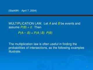
(Stat49N - April 7, 2004) MULTIPLICATION LAW. Let Aand B be events and assume P(B) 0. Then P(A B) = P(A | B) P(B) The multiplication law is often useful in finding the probabilities of intersections, as the following examples illustrate.
Example A. An urn contains three red balls and one blue ball. Two balls are selected without replacement. What is the probability that they are both red? Let R1 and R2denote the events that a red ball is drawn on the first trial and on the second trial, respectively. From the multiplication law, P(R1R2) = P(R1) P(R2 | R1) P(R1) is clearly ¾ , and if a red ball has been removed on the first trial, there are two red balls and one blue ball left. Therefore P(R1R2) =2/3. Thus P(R1R2) =½ .
LAW OF TOTAL PROBABILITY. Let B1, B2, … Bn be such that U Bi = and Bi Bj = for i j, with P(Bi) > 0 for all i. Then, for any event A, P(A) = P(A | Bi) P(Bi) n i=1 n i=1
EXAMPLE C. Referring to Example A, what is the probability that a red ball is selected on the second draw? The answer may or may not be intuitively obvious – that depends on your intuition. On the one hand, you could argue that it is “clear from symmetry” that P(R2) = P(R1) = ¾. On the other hand, you could say that it is obvious that a red ball is likely to be selected on the first draw, leaving fewer red balls for the second draw, so that P(R2) < P(R1). The answer can be derived easily by using the law of total probability.
P(R2) = P(R2 | R1) P(R1) + P(R2 | B1) P(B1) = 2/3 x 3/4 + 1 x 1/4 = 3/4 where B1 denotes the event that a blue ball is drawn on the first trial. BAYES’ RULE. Let A and B1, …, Bnbe events where the Bi are disjoint, U Bi = , and P(Bi) > 0 for all i. Then P(Bj | A) = ----------------------------------- n i=1 P(A | Bj) P(Bj) P(A | Bi) P(Bi) n i=1
INDEPENDENCE. Intuitively, we would say that two events, A and B, are independent if knowing that one had occurred gives us no information about whether the other had or will occur; that is, P(A | B) = P(A) and P(B | A) = P(B). Now, if P(A) = P(A | B) = --------------- then P(A B) = P(A) P(B) We will use this last relation as the definition of independence. Note that it is symmetric in A, and B and does not require the existence of a conditional probability; that is, P(B) can be 0. DEFINITION. A and B are said to be independent events if P(A B) = P(A) P(B). P(A B) P(B)
EXAMPLE a. A card is selected randomly from a deck. Let A denote the event that it is an ace and D the event that it is a diamond. Knowing that the card is an ace gives no information about its suit. Checking formally that the events are independent, we have P(A) = 4/52 = 1/13 and P(D) = 1/4. Also, AD is the event that the card is the ace of diamonds and P(A D) =1/52. Since P(A) P(D) = (1/4) x (1/13) = 1/52, the events are in fact independent.
EXAMPLE c. A fair coin is tossed twice. Let A denote the event of heads on the first toss, B the event of heads on the second toss, and C the event that exactly one head is thrown. A and B are clearly independent, and P(A) = P(B) = P(C) = .5. To see that A and C are independent, we observe that P(C | A) = .5. But P(A B C) = 0 P(A) P(B) P(C) To encompass situations such as that in Example c, we define a collection of events, A1, A2, … An, to be mutually independent if for any subcollection, Ai , …, Ai , P(Ai ··· Ai ) = P(Ai ) ··· P(Ai ) m 1 1 m m 1
Discrete Random Variables. • A random variable is essentially a random number. We will be interested in random numbers that are determined by experiments. As motivation for a definition, let us consider an example. A coin is thrown three times, and the sequence of heads and tails is observed; thus, • = { hhh, hht, htt, hth, ttt, tth, thh, tht } • Examples of random variables associated with are • the total number of heads, • the total number of tails, and • the number of heads minus the number of tails. • Each of these is a real-valued function defined on ; that is, • each is a rule that assigns a real number to every point . Since the outcome in is random, the corresponding number is random as well.
In general, a random variable is a function from to the real numbers. Since the outcome of the experiment for which is the sample space is random, the number produced by the function is random as well. It is conventional to denote random variables by italic uppercase letters from the end of the alphabet. For example, we might define X to be the total number of heads in the experiment described above. A discrete random variable is a random variable that can take on only a finite or at most a countably infinite number of values. The random variable X just defined is a discrete random variable since it can take on only the values 0, 1, 2, and 3. For an example of a random variable that can take on a countably infinite number of values, consider an experiment that consists of tossing a coin until a head turns up and defining Y to be the total number of tosses. The possible values of Y are 0, 1, 2, 3, … . In general, a countably infinite set is one that can be put into one-to-one correspondence with the integers.
If the coin is fair, then each of the outcomes in above has probability 1/8, from which the probabilities that X takes on the values 0, 1, 2, and 3 can be easily computed: P(X = 0) = 1/8 P(X = 1) = 3/8 P(X = 2) = 3/8 P(X = 3) = 1/8
Generally, the probability measure on the sample space determines the probabilities of the various values of X; if those values are denoted by x1, x2, …, then there is a function p such that p(xi)=P(X=xi) and i p(xi) = 1. This function is called the probability mass function, or the frequency function, of the random variable X. Figure below shows a graph of p(x) for the coin tossing experiment. The frequency function describes completely the probability properties of the random variable.
In addition to the frequency function, it is sometimes useful to use the cumulative distribution function (cdf) of a random variable, which is defined to be F(x) = P(X x), - < x < Cumulative distribution functions are usually denoted by uppercase letters and frequency functions by lowercase letters. Figure below is a graph of the cumulative distribution function of the random variable X of the preceding paragraph. Note that the cdf jumps where p(x) > 0 and that the jump at xiis p(xi).
It is useful to define here the concept of independence of random variables. In the case of two discrete random variables X and Y, taking on possible values x1, x2, … and y1, y2, …, X and Y are said to be independent if, for all i and j, P (X = xiand Y = yj) = P(X = xi) P(Y = yj) The definition is extended to collections of more than two discrete random variables in the obvious way; for example, X, Y, and Z are said to be mutually independent if, for all i, j, and k, P (X = xi ,Y = yj , Z = zk) = P(X = xi) P(Y = yj) P(Z = zk) We next discuss some common discrete distributions that arise in applications.
Bernoulli Random Variables. A Bernoulli random variable takes on only two values: 0 and 1, with probabilities 1 – p and p, respectively. Its frequency function is thus p(1) = p p(0) = 1 – p p(x) = 0, if x 0 or x 1 An alternative and sometimes useful representation of this function is p(x){ px (1 – p) 1-x , if x = 0 or x = 1 0, otherwise
If A is an event, then the indicator random variable, IA, takes on the value 1 if A occurs and the value 0 if A does not occur: IA () = { IA is a Bernoulli random variable. In applications, Bernoulli random variables often occur as indicators. A Bernoulli random variable might take on the value 1 or 0 according to whether a guess was a success or a failure. 1, if A 0, other wise
The Binomial Distribution. Suppose that n independent experiments, or trials, are performed, where n is a fixed number, and that each experiment results in a “success” with probability p and a “failure” with probability 1 – p. The total number of successes, X, is a binomial random variable with parameters n and p. For example, a coin is tossed 10 times and the total number of heads is counted (“head” is identified with “success”). The probability that X = k, or p(k), can be found in the following way. Any particular sequence of k successes occurs with probability pk (1 – p)n-k, from the multiplication principle. The total number of such sequences is ( ) , since there are ( ) ways to assign k successes to n trials. Thus, p(k) = ( ) pk (1 – p)n-k n k n k n k
Two binomial frequency functions are shown in Figure 2-3. Note how the shape varies as a function of p.
EXAMPLE. Tay-Sachs disease is a rare but fatal disease of genetic origin occurring chiefly in infants and children, especially those of Jewish, eastern European extraction. If a couple are both carriers of Tay-Sachs disease, a child of theirs has probability .25 of being born with the disease. If such a couple has four children, what is the frequency function for the number of children that will have the disease?
We assume that the four outcomes are independent of each other, so, if X denotes the number of children with the disease, p(k) = ( ) .25k .754-k, k = 0, 1, 2, 3, 4 These probabilities are given in the following table: k p(k) ------------------ 0 .316 1 .422 2 .211 3 .047 4 .004 4 k


![[b] [p]](https://cdn1.slideserve.com/3197655/slide1-dt.jpg)


![定理 1 4 .1:[ R;+, * ] 为环,则对任 a,b R , 有: (1) a *0=0*a=0 (2)a *(-b)=(-a)*b=-(a*b) (3) (-a)*(-b)=a*b](https://cdn2.slideserve.com/4799316/slide1-dt.jpg)