Download
1 / 34
340 likes | 493 Views
A Constraint Generation Approach to Learning Stable Linear Dynamical Systems. Sajid M. Siddiqi Byron Boots Geoffrey J. Gordon. Carnegie Mellon University. NIPS 2007 poster W22. Objective.

E N D
A Constraint Generation Approach to Learning Stable Linear Dynamical Systems Sajid M. SiddiqiByron BootsGeoffrey J. Gordon Carnegie Mellon University NIPS 2007poster W22
Objective • Learn parameters of a Linear Dynamical System from data while ensuring a stable dynamics matrix Amore efficiently and accurately than previous methods
Our Approach • Formulate an approximation of the problem as a semi-definite program (SDP) • Start with a quadratic program (QP)relaxation of this SDP, and incrementally add constraints • Because the SDP is an inner approximation of the problem, we reach stabilityearly, before reaching the feasible set of the SDP • We interpolate the solution to return the best stable matrix possible
Outline • Linear Dynamical Systems • Stability • Convexity • Constraint Generation Algorithm • Empirical Results • Conclusion
Application: Dynamic Textures1 • Videos of moving scenes that exhibit stationarity properties • Can be modeled by a Linear Dynamical System • Learned models can efficiently simulate realistic sequences • Applications: compression, recognition, synthesis of videos • But there is a problem … steam river fountain 1 S. Soatto, D. Doretto and Y. Wu. Dynamic Textures. Proceedings of the ICCV, 2001
Linear Dynamical Systems • Input data sequence • Assume a latent variable that explains the data • Assume a Markov model on the latent variable
Linear Dynamical Systems2 • State and observation updates: • Dynamics matrix: • Observation matrix: 2 Kalman, R. E. (1960). A new approach to linear filtering and prediction problems. Trans.ASME-JBE
Learning Linear Dynamical Systems • Suppose we have an estimated state sequence • Define state reconstruction error as the objective: • We would like to learn such that i.e.
Subspace Identification3 • Subspace ID uses matrix decomposition to estimate the state sequence • Build a Hankel matrixD of stacked observations 3 P.Van Overschee and B. De Moor Subspace Identification for Linear Systems. Kluwer, 1996
Subspace ID with Hankel matrices Stacking multiple observations in D forces latent states to model the future e.g. annual sunspots data with 12-year cycles = k = 12 k = 1 t t First 2 columns of U
Subspace Identification3 • In expectation, the Hankel matrix is inherently low-rank! • Can use SVD to obtain the low-dimensional state sequence For D with k observations per column, = 3 P.Van Overschee and B. De Moor Subspace Identification for Linear Systems. Kluwer, 1996
Training LDS models • Lets train an LDS for steam textures using this algorithm, and simulate a video from it! = [ …] xt2 R40
Simulating from a learned model xt t The model is unstable
Notation • 1 , … , n : eigenvalues of A (|1| > … > |n| ) • 1,…,n: unit-length eigenvectors of A • 1,…,n: singular values of A (1 > 2 > … n) • S : matrices with |1| · 1 • S : matrices with1 · 1
Stability • a matrix A is stable if |1|· 1, i.e. if • Why? matrix of eigenvectors eigenvalues in decreasing order of magnitude
Stability • We would like to solve xt(1), xt(2) |1| = 0.3 xt(1), xt(2) |1| = 1.295 s.t.
Stability and Convexity • The state space of a stable LDS lies inside some ellipse • The set of matrices that map a particular ellipse into itself (and hence are stable) is convex • If we knew in advance which ellipse contains our state space, finding A would be a convex problem. But we don’t • …and the set of all stable matrices is non-convex ? ? ?
Stability and Convexity • So, S is non-convex! • Lets look at S instead … • S is convex • S µS • Previous work4exploits these properties to learn a stable A bysolving an SDP for the problem: A1 A2 s.t. 4 S. L. Lacy and D. S. Bernstein. Subspace identification with guaranteed stability using constrained optimization. In Proc. of the ACC (2002), IEEE Trans. Automatic Control (2003)
Simulating from a Lacy-Bernstein stable texture model xt t Model is over-constrained.Can we do better?
Our Approach • Formulate the S approximation of the problem as a semi-definite program (SDP) • Start with a quadratic program (QP)relaxation of this SDP, and incrementally add constraints • Because the SDP is an inner approximation of the problem, we reach stabilityearly, before reaching the feasible set of the SDP • We interpolate the solution to return the best stable matrix possible
The Algorithm objective function contours • A1: unconstrained QP solution (least squares estimate) • A2:QP solution after 1 constraint (happens to be stable) • Afinal:Interpolation of stable solution with the last one • Aprevious method:Lacy Bernstein (2002)
Quadratic Program Formulation Constraints are of the form
Simulating from a Constraint Generation stable texture model xt t Model captures more dynamics and is still stable
Empirical Evaluation • Algorithms: • Constraint Generation – CG (our method) • Lacy and Bernstein (2002) –LB-1 • finds a 1· 1 solution • Lacy and Bernstein (2003)–LB-2 • solves a similar problem in a transformed space • Data sets • Dynamic textures • Biosurveillance
Reconstruction error • Steam video % decrease in objective (lower is better) number of latent dimensions
Running time • Steam video Running time (s) number of latent dimensions
Reconstruction error • Fountain video % decrease in objective (lower is better) number of latent dimensions
Running time • Fountain video Running time (s) number of latent dimensions
Conclusion • A novel constraint generation algorithm for learning stable linear dynamical systems • SDP relaxation enables us to optimize over a larger set of matrices while being more efficient • Future work: • Adding stability constraints to EM • Stable models for more structured dynamic textures