Streaming Algorithms and Approximations for Geometric Problems
This talk discusses the implementation of streaming algorithms for geometric problems, emphasizing single-pass processing, bounded storage, and fast computational techniques. It covers approaches like k-center and k-median problems and their approximations in geometric spaces using core-sets, which are efficient subsets of data that retain essential characteristics. The talk highlights the application of techniques such as trees for computation and randomized embeddings, enabling efficient processing of vast data through a reduced representation without losing significant information.

Streaming Algorithms and Approximations for Geometric Problems
E N D
Presentation Transcript
Approximations and Streaming Algorithms for Geometric Problems Piotr Indyk MIT
Computational Model • Single* pass over the data: e1, e2, …,en • Bounded storage • Fast processing time per element *For the purpose of this talk
Streaming Data Types • Vector problems: • Stream defines an array of numbers • Maintain stats of the array, e.g., median • Metric problems • Clustering • Graph problems, Text problems • Geometric Problems [this talk]
Geometric Data Stream Algorithms as Data Structures • Data structures that support: • Insert(p) to P • Possibly: Delete(p) from P • Compute(P) • Use space that is sub-linear in |P|
Clustering in Geometric Spaces • Problems: • k-center [Charikar-Chekuri-Feder-Motwani’97] • k-median [Guha-Mishra-Motwani-O’Callaghan’00, Meyerson’01, Charikar-O’Callaghan-Panigrahy’03] • Bounds: • poly(k,log n) space • O(1)-approximation
k-median/k-center • k is given • Goal: choose k medians/centers to minimize: • k-median: the sum of the distances • k-center: the max distance
Geometric Space • Bounds: • poly(k,log n) space • (1+)-approximation • Problems: • Diameter, Minimum Enclosing Ball [Agarwal-Har-Peled’01, Feigenbaum-Kannan-Zhang’02, Cormode-Muthukrishnan’02, Hershberger-Suri’04] • k-center [Agarwal-HarPeled’01, Agarwal-HarPeled-Varadarajan’04] • k-median [HarPeled-Mazumdar’04] • Range searching via -approximations: • [Suri-Toth-Zhou’04] • [Bagchi-Chaudhary-Eppstein-Goodrich’04] • …
Dominant Approach: Merge and Reduce • Main ideas: • Design an (off-line) algorithm that converts the input into a “sketch”: • Small size • Sufficient to solve the problem • A sketch of sketches is a sketch • Partition the input in a tree-like fashion • Simulate tree computation in small space • Technique can traced back to ancient times i.e., 80’s [Munro-Paterson’80]
Tree Computation p1 p2 p3 p4 p5 p6 p7 p8 p9 p10 p11 p12 p13 p14 p15 p16
Analysis • Space: (sketch size)*log n • Time: sketch computation time • Question: Where do sketches come from ?
Idea I: solution=sketch • Consider k-median • [GMMO’00] : approximate k-median of approximate weighted k-medians is an approximate k-median • Result: • Constant depth tree • Space: kn, >0 • O(1) -approximation • Works for any metric space 3 2 1 3 2 1 k=3
Use the solution, ctd. • -Approximations: find a subset SP , such that for any rectangle/halfspace/etc R, |RS|/|S|=|RP|/|P| • [Matousek] : approximation of a union of approximations is an approximation • [BCEG’04] : convert it into streaming algorithm, applications • 1/2space • [STZ’04] : better/optimal bounds for rectangles and halfspaces
Idea 2: Core-Sets [AHP’01] • Assume we want to minimize CP(o) • SP is an -core-set for P, if for any o, and a set T: CPT (o) = (1 ±) CST (o) • Note: this must hold for all o, not just the optimal one o P
Example: Core-set for MEB • Compute extremal points: • Choose “densely” spaced direction v1 …vk • I.e., for any u there is vi such that u*vi ≥ ||u||2 / (1+) • For each direction maintain extremal point • k=O(1/)(d-1)/2suffice
Stream Algorithms via Core-sets • Diameter/MEB/width: O(1/)(d-1)/2 log n space [AHP’01] • k-center: O(k/d) log n [HP’01] • k-median: • O(k/d) log n [HPM’04] • O(k2/d) [HPK’05] • O(k2d log6 n/) [Chen’05] • O(d3/7), k=1 [Indyk’05] • Faster algorithms and other results
Limitations • Small core-sets might not exist • Do not support deletions
Insertions and Deletions • Technique: • Reduction of geometric problems to vector problems • Use of randomized linear embeddings • Problems: • Maintaining histograms of the data • Classic geometric problems (matching, MST, clustering etc)
Streaming Algorithms for Vector Problems • Norm estimation: • Stream elements: (i,b) , i=1…m • Interpretation: xi=xi+b • Want to maintain ||x||p • Why ? Examples: • ||x||pp =Σi xip = #non-zero coordinates in x, as p0 • … • How ?
Dimensionality reduction • x is an m-dimensional vector • A is a “random” m times k matrix, k “small” • Store Ax • Recover (1±)||x||2 from Ax (with prob. 1-1/N ) • [Alon-Matias-Szegedy’96] • Estimator: median[ (A1x)2+..+ (Ac x)2, (Ac+1x)2+..+ (A2cx)2,..]1/2 , c=1/2 , k=c log N • A: constructed from 4-wise independent random variables • [Johnson-Lindenstrauss’85] • Estimator: ||Ax||2 • A: each entry independently drawn from e.g. Gaussian distribution • constructed using Nisan’s PRG [Indyk’00] • [Indyk’00] • Estimator: median[ (A1x),…, (Ak x) ] • A: as above • Works for ||x||p any p(0,2] (using p-stable distributions)
What it means • To know ||x||2, suffices to know Ax • Can maintain Ax when the coordinates are incremented: A(x+ bei)=Ax+ bA ei Ax A x
Applications of Vector Approach • Histograms/wavelet approximation • Classic geometric problems (matching, MST, clustering etc)
Histograms • View x as a function x:[1…n] [1…M] • Approximate it using piecewise constant function h, with B pieces (buckets) • Problem can be formulated in 2D as well (buckets become rectangular tiles)
Results: 1D • [Gilbert-Guha-Indyk-Kotidis-Muthukrishnan-Strauss’02] : • Maintains h with B pieces such that ||x-h||2 ≤ (1+)||x-hOPT||2 • Under increments/decrements of x • Space: poly(B,1/,log n) • Time: poly(B,1/,log n)
Results: 2D • [Thaper-Guha-Indyk-Koudas’02] : • Maintains h with Blog (nM) tiles such that ||x-h||2 ≤ (1+)||x-hOPT||2 • Under increments/decrements of x • Space/Update time: poly(B,1/,log n) • Histogram reconstruction time: poly(B,1/, n) • [Muthukrishnan-Strauss’03] : • Maintains h with 4B tiles • Time: poly(B,1/, log(nM))
Minimum Weight Bi-chromatic Matching • Estimate the cost of MWBM
Minimum Weight Matching • Estimate the cost of MWM
Minimum Spanning Tree • Estimate the cost of MST
Facility Location • Goal: choose a set F of facilities to minimize the • sum of the distances to nearest facility plus • the number of facilities times f • Again, report the cost
Approach [Indyk’04] • Assume P{1…}2 • Reduce to vector problems • Impose square grids G0…Gk, with side lengths 20,21, …, 2k, shifted at random. • For each square cell c in Gi, let nP(c) be the number of points from P in c. • The algorithms will maintain certain statistics over nP(.), which will allow it to approximately solve the problems 1 2 1 3 1 5 1 1
Estimators • MST: ∑i 2i ∑c Gi [nP(c)>0] • MWM: ∑i 2i∑c Gi [nP(c) is odd] • MWBM: ∑i 2i ∑c Gi |nG(c)-nB(c)| • Fac. Loc.: ∑i 2i∑c Gi min[nP(c), Ti] • K-median: ∑i 2i∑c Gi - B(Q, 2^i)nP(c) (given medians Q) Maintain #non-zero entries in nP[FM’85] Maintain L1 difference [I’00]
Results [Frahling-Indyk-Sohler’05] […, Charikar’02, …] [Frahling-Sohler’05] Space: (log +log n + K )O(1)
XYZ Space: (K+log + log n)O(1)
Probabilistic embeddings into HST’s T 1 2 1 3 1 5 1 1 • Known[Bartal’96, Charikar-Chekuri-Goel-Guha-Plotkin’98]: • ||p-q|| ≤ Dtree (p,q) • E[ Dtree(p,q) ] ≤ ||p-q|| * O(log )
MST • E[Cost(MST in T)] ≤ O(log ) Cost(MST) • Cost(MST in T) Cost(T) • How to compute Cost(T) ? • Sum over all levels i, of the #nodes at i, times 2i • Node c exists iff ni(c)>0 1 2 1 3 1 5 1 1
Matching • Algorithm: • Match what you can at the current level • Odd leftovers wait for the next level • Repeat • Optimal on the HST • Cost=∑i 2i ∑c Gi [nP(c) is odd] 1 0 1 1 1 0 1 1 0
Conclusions • Algorithms for geometric data streams • Insertions-only: merge and reduce, coresets • Insertions and deletions: randomized linear embeddings
Open Problems • Matchings, Facility Location, etc: • Replace log by O(1) or even 1+ • Possible for: • MST [Frahling-Indyk-Sohler’05] • k-median [Frahling-Sohler’05] • Related to computing bi-chromatic matching [Agarwal-Varadarajan’04] • Min-sum clustering ?
Open Problems • High dimensions: • Diameter: • 21/2-approx, O(d2 n1/2 ) space, follows from [Goel-Indyk-Varadarajan’01] • c-approx, O( dn1/(c2 - 1) )[Indyk’03] • Conjecture: 21/2-approx, O(d polylog n) space • Min-width cylinder: 18-approx, O(d) space [Chan’04]
Open Problems • Range queries: • General lower bounds ? (Not just for - approximations) • (1/2) -bit bound for general queries follows from LB for dot product [Indyk-Woodruff’03] and is tight (for randomized algorithms) • What about e.g., half-space queries ? O(1/4/3) is known [STZ’04] • Other problems [STZ’04]