Introduction to Statistics − Day 3

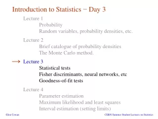
1. Introduction to Statistics − Day 3 Lecture 1 Probability Random variables, probability densities, etc. Lecture 2 Brief catalogue of probability densities The Monte Carlo method. Lecture 3 Statistical tests Fisher discriminants, neural networks, etc Goodness-of-fit tests Lecture 4 Parameter estimation Maximum likelihood and least squares Interval estimation (setting limits) → Glen Cowan CERN Summer Student Lectures on Statistics

2. Statistical tests (in a particle physics context) Suppose the result of a measurement for an individual event is a collection of numbers x1 = number of muons, x2 = mean pt of jets, x3 = missing energy, ... follows some n-dimensional joint pdf, which depends on the type of event produced, i.e., was it For each reaction we consider we will have a hypothesis for the pdf of , e.g., etc. Often call H0 the signal hypothesis (the event type we want); H1, H2, ... are background hypotheses. Glen Cowan CERN Summer Student Lectures on Statistics etc.

3. Selecting events Suppose we have a data sample with two kinds of events, corresponding to hypotheses H0 and H1 and we want to select those of type H0. Each event is a point in space. What ‘decision boundary’ should we use to accept/reject events as belonging to event type H0? H1 Perhaps select events with ‘cuts’: H0 accept Glen Cowan CERN Summer Student Lectures on Statistics

4. Other ways to select events Or maybe use some other sort of decision boundary: linear or nonlinear H1 H1 H0 H0 accept accept How can we do this in an ‘optimal’ way? What are the difficulties in a high-dimensional space? Glen Cowan CERN Summer Student Lectures on Statistics

5. Test statistics Construct a ‘test statistic’ of lower dimension (e.g. scalar) Try to compactify data without losing ability to discriminate between hypotheses. We can work out the pdfs Decision boundary is now a single ‘cut’ on t. This effectively divides the sample space into two regions, where we accept or reject H0. Glen Cowan CERN Summer Student Lectures on Statistics

6. Significance level and power of a test Probability to reject H0 if it is true (error of the 1st kind): (significance level) Probability to accept H0 if H1 is true (error of the 2nd kind): (1 - b = power) Glen Cowan CERN Summer Student Lectures on Statistics

7. Efficiency of event selection Probability to accept an event which is signal (signal efficiency): Probability to accept an event which is background (background efficiency): Glen Cowan CERN Summer Student Lectures on Statistics

8. Purity of event selection Suppose only one background type b; overall fractions of signal and background events are ps and pb (prior probabilities). Suppose we select events with t < tcut. What is the ‘purity’ of our selected sample? Here purity means the probability to be signal given that the event was accepted. Using Bayes’ theorem we find: So the purity depends on the prior probabilities as well as on the signal and background efficiencies. Glen Cowan CERN Summer Student Lectures on Statistics

9. Constructing a test statistic How can we select events in an ‘optimal way’? Neyman-Pearson lemma (proof in Brandt Ch. 8) states: To get the lowest eb for a given es (highest power for a given significance level), choose acceptance region such that where c is a constant which determines es. Equivalently, optimal scalar test statistic is Glen Cowan CERN Summer Student Lectures on Statistics

10. Why Neyman-Pearson doesn’t always help The problem is that we usually don’t have explicit formulae for the pdfs Instead we may have Monte Carlo models for signal and background processes, so we can produce simulated data, and enter each event into an n-dimensional histogram. Use e.g. M bins for each of the n dimensions, total of Mn cells. But n is potentially large, →prohibitively large number of cells to populate with Monte Carlo data. Compromise: make Ansatz for form of test statistic with fewer parameters; determine them (e.g. using MC) to give best discrimination between signal and background. Glen Cowan CERN Summer Student Lectures on Statistics

11. Linear test statistic Ansatz: Choose the parameters a1, ..., an so that the pdfs have maximum ‘separation’. We want: ms g (t) mb large distance between mean values, small widths ss sb t → Fisher: maximize Glen Cowan CERN Summer Student Lectures on Statistics

12. Fisher discriminant Using this definition of separation gives a Fisher discriminant. H1 Corresponds to a linear decision boundary. H0 accept Equivalent to Neyman-Pearson if the signal and background pdfs are multivariate Gaussian with equal covariances; otherwise not optimal, but still often a simple, practical solution. Glen Cowan CERN Summer Student Lectures on Statistics

13. Nonlinear test statistics The optimal decision boundary may not be a hyperplane, →nonlinear test statistic H1 Multivariate statistical methods are a Big Industry: Neural Networks, Support Vector Machines, Kernel density methods, ... H0 accept Particle Physics can benefit from progress in Machine Learning. Glen Cowan CERN Summer Student Lectures on Statistics

14. Neural network example from LEP II Signal: e+e-→ W+W- (often 4 well separated hadron jets) Background: e+e-→ qqgg (4 less well separated hadron jets) ← input variables based on jet structure, event shape, ... none by itself gives much separation. Neural network output does better... (Garrido, Juste and Martinez, ALEPH 96-144) Glen Cowan CERN Summer Student Lectures on Statistics

15. Testing goodness-of-fit for a set of Suppose hypothesis H predicts pdf observations We observe a single point in this space: What can we say about the validity of H in light of the data? Decide what part of the data space represents less compatibility with H than does the point more compatible with H less compatible with H (Not unique!) Glen Cowan CERN Summer Student Lectures on Statistics

16. p-values Express ‘goodness-of-fit’ by giving the p-value for H: p = probability, under assumption of H, to observe data with equal or lesser compatibility with H relative to the data we got. This is not the probability that H is true! In frequentist statistics we don’t talk about P(H) (unless H represents a repeatable observation). In Bayesian statistics we do; use Bayes’ theorem to obtain where p (H) is the prior probability for H. For now stick with the frequentist approach; result is p-value, regrettably easy to misinterpret as P(H). Glen Cowan CERN Summer Student Lectures on Statistics

17. p-value example: testing whether a coin is ‘fair’ Probability to observe n heads in N coin tosses is binomial: Hypothesis H: the coin is fair (p = 0.5). Suppose we toss the coin N = 20 times and get n = 17 heads. Region of data space with equal or lesser compatibility with H relative to n = 17 is: n = 17, 18, 19, 20, 0, 1, 2, 3. Adding up the probabilities for these values gives: i.e. p = 0.0026 is the probability of obtaining such a bizarre result (or more so) ‘by chance’, under the assumption of H. Glen Cowan CERN Summer Student Lectures on Statistics

18. The significance of an observed signal Suppose we observe n events; these can consist of: nb events from known processes (background) ns events from a new process (signal) If ns, nb are Poisson r.v.s with means s, b, then n = ns + nb is also Poisson, mean = s + b: Suppose b = 0.5, and we observe nobs = 5. Should we claim evidence for a new discovery? Give p-value for hypothesis s = 0: Glen Cowan CERN Summer Student Lectures on Statistics

19. The significance of a peak Suppose we measure a value x for each event and find: Each bin (observed) is a Poisson r.v., means are given by dashed lines. In the two bins with the peak, 11 entries found with b = 3.2. The p-value for the s = 0 hypothesis is: Glen Cowan CERN Summer Student Lectures on Statistics

20. The significance of a peak (2) But... did we know where to look for the peak? → give P(n ≥ 11) in any 2 adjacent bins Is the observed width consistent with the expected x resolution? → take x window several times the expected resolution How many bins  distributions have we looked at? →look at a thousand of them, you’ll find a 10-3 effect Did we adjust the cuts to ‘enhance’ the peak? →freeze cuts, repeat analysis with new data How about the bins to the sides of the peak... (too low!) Should we publish???? Glen Cowan CERN Summer Student Lectures on Statistics

21. Wrapping up lecture 3 We looked at statistical tests and related issues: discriminate between event types (hypotheses), determine selection efficiency, sample purity, etc. Some modern (and less modern) methods were mentioned: Fisher discriminants, neural networks, support vector machines,... We also talked about goodness-of-fit tests: p-value expresses level of agreement between data and hypothesis Next we’ll turn to the second main part of statistics: parameter estimation Glen Cowan CERN Summer Student Lectures on Statistics