Download
1 / 39
400 likes | 600 Views
CS314: Formal languages and automata theory L. Nada ALZaben. Chapter 7 . Time Complexity. Quick Note. don’t forget to read chapter 6section 6.1 and 6.2 Always check the blog for new updates: Cs314pnu.wordpress.com. Quick revision. Lecture #16.

E N D
CS314: Formal languages and automata theoryL. Nada ALZaben Chapter 7. Time Complexity
Quick Note • don’t forget to read chapter 6section 6.1 and 6.2 • Always check the blog for new updates: Cs314pnu.wordpress.com Computer Science Department
Quick revision Lecture #16 • The theory of computation is divided over three parts: • Part1: Automata • Part2: Computability • Part3: Complexity. → Computability → Automata → Complexity Problem can be solved (true – false) Ch:3-6 Computer problems (hard or easy) Ch:7- end of book Deal with definitions and properties of mathematical model (FA – CFG) Ch:1-2
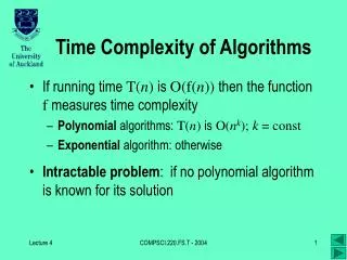
Time complexity • Even when a problem is decidable and computationally solvable it may not be solvable in practice if the solution requires an inordinate amount of time and space. • Complexity theory: is an investigation of the time, memory or other resources required for solving computational problems.
7.1 measuring complexity • How much time does a Turing Machine tape need to decide language A? • Describe TM ,M1, at a low level and count the number of steps that m1 uses when it runs.
7.1 measuring complexity • The number of steps that an algorithm uses on a particular input may depend on several parameters but for simplicity we compute as a function of the length of the string representing the inputs. • In worst-case analysis consider the longest running time of all inputs of a particular length. • In average-case analysis consider the average running time of all inputs of a particular length.
Big-O and Small-O notation • Asymptotic analysis one convenient form of estimation. By just considering the highest order term of the expression and ignore any coefficient and any lower order term . • For example: • The asymptotic notation or Big-O notation is
Big-O and Small-O notation • Example: • Example: • Example: Let f3(n) be the function
Big-O and Small-O notation • Example:
Analyzing algorithms Lecture #17
Analyzing algorithms • Time () contains all languages that can be decided with time complexity O () so we can say for the language A:
Analyzing algorithms • Machine M2 uses different algorithm to decide on language A to give a shorter time than M1.
Analyzing algorithms • Machine M3 uses second tape and uses a different algorithm to decide on language A (linear time )
Complexity Relationships among models • The choice of computational model can effect the time complexity of languages. • Three models used: • The single tape TM. • The multitape TM. • Nondeterministic TM
7.2 The Class P Lecture #18 • Previous theorems show two important distinction: • Polynomial difference in running time is small • Exponential difference in running time is large. • Ex: when n=1000. • Polynomial Time: • Algorithms are fast enough for many purposes unlike the Exponential Time. (ex. Brute-force search) • Polynomially equivalent. (ex. Deterministic single and multi tape TM’s)
7.2 The Class P • The class P plays an important role because: • P is invariant for all models of computation that are Polynomially equivalent to the deterministic single-tape TM. • P roughly corresponds to the class of problems that are realistically solvable on a computer.
7.2 The Class P • Giving a polynomial time algorithm in a high-level description with out referring to a particular computation model or even details of tapes and head motion. • Algorithms are described with numbered stages. • Stage of an algorithm might be implemented by several steps in TM. • To give the polynomial time of an algorithm : • Give the polynomial upper bound on the number of stages that an algorithm uses when running on input of length n. • Examine the individual stages to be sure that each can be implemented in polynomial time on a deterministic model.
7.2 The Class P • Examples of problems in P: • Encoding of graphs – an encoding of a graph is a list of its nodes and edges. (adjacency matrix : the (i,j)th entry is 1 if there is an edge from I to j) and 0 when not. • The running time on graphs is computed by the number of nodes instead of the size of the node. So it gives a polynomial time on the number of nodes and then it is polynomial in the size of the input. • In the directed graph G contains nodes s and t the PATH problem is to find a directed path between the nodes s and t. as in the figure.
7.2 The Class P • Examples of problems in P: PATH problem is there a path from s to t?
7.2 The Class P • Examples of problems in P: RELPRIME problem is deciding if two numbers are relatively prime?
7.2 The Class P Greatest common divisor gcd(x,y)
7.2 The Class P • Using a powerful technique called dynamic programming
7.3 The Class NP • We previously produced the polynomial time and stated its is faster than the exponential one. • Some problems was solved by brute-force search and we had an alternative solution to have it in polynomial time • Sometimes this can not be obtain. • Example: Hamiltonian path in directed graph G is a directed path that goes through each node exactly once.
7.3 The Class NP • By modifying the PATH algorithm that was solved by brute-force search (just before it was solved by a polynomial time) we can obtain an algorithm that can decide if the path is Hamiltonian. • The HAMPATH problem have feature called polynomial verifiability which is used for its complexity. • Although deciding if a path is Hamiltonian requires an exponential time it may be solved and proven to be existed. This is called verifying. • Verifying the existence of Hamiltonian path is easier than determining its existence. • Example: of polynomial verifiability is compositeness. • (composite number is a none prime number)
7.3 The Class NP • HAMPATH and COMPOSITES are members of NP. • COMPOSITES are members of P too. • P is a subset of NP.
7.3 The Class NP • NTM that decides HAMPATH problem in NP: • Although each stage is decided in a polynomial time this algorithm runs in nondeterministic polynomial time.
7.3 The Class NP • Example of problem in NP: • A clique in an undirected graph is a sub-graph where every two nodes are connected by an edge. • A k-clique is a clique that contain k nodes.
7.3 The Class NP • Example