
Error Backpropagation
E N D
Presentation Transcript
Error Backpropagation • All learning algorithms for (layered) feed-forward networks are based on a technique called error backpropagation • This is a form corrective supervised learning which consists of two phases. In the first (for-ward) phase the output of each neuron is computed, in the second (backward) phase the partial derivatives of the error function with respect to the weights are computed, where-after the weights are updated Rudolf Mak TU/e Computer Science
Approach • The approach we take • is a minor variation of the one in: R. Rojas, • Neural Networks, Springer, 1996. • applies to general feed-forward networks • allows distinct activation functions for each of • the neurons • uses a graphical method called B-diagrams • to illustrate how partial derivatives of the error • function can be computed Rudolf Mak TU/e Computer Science
General Feed-forward Networks • A general feed-forward network consists of • n input nodes (numbered 1, … , n) • l hidden neurons (numbered n+1, … , n+l) • m output neurons (numbered n+l+1, … , n+l+m) • a set of connections such that the network does • not contain cycles. Hence the hidden neurons • can be topologically sorted, i.e. numbered such • that (i, j) is a connection, iff • i < j and n < j and i < n+l+1. Rudolf Mak TU/e Computer Science
B-diagrams • A B-diagram is a directed acyclic network containing four types of nodes • Fan-in nodes • Fan-out nodes • Product nodes • Function nodes • The forward phase computes function composition, the backward phase computes partial derivatives. Rudolf Mak TU/e Computer Science
B-diagram (fan-in node) Forward phase Backward phase Rudolf Mak TU/e Computer Science
d ( |y ) y 1 1 ( |y ) d 1 y 2 1 2 S d ( |x) x 1 d ( |y ) y n n B-diagram (fan-out node) Forward phase Backward phase Rudolf Mak TU/e Computer Science
d d ( |x) ( |y) x y B-diagram (product node) Forward phase Backward phase Rudolf Mak TU/e Computer Science
d d ( |x) ( |y) x y B-diagram (function node) Forward phase Backward phase Rudolf Mak TU/e Computer Science
g(f(x)) f(x) g’(f(x))f ’(x) g’(f(x)) Chain-rule x 1 (g f)(x) = g(f(x)) (g f)’(x) = g’(f(x))f ’(x) Rudolf Mak TU/e Computer Science
Remark Note that the product node, the fan-in node, and the function node are all special cases of a more general node for functions with an arbitrary num- ber of arguments that stores all partial derivates. f (x1, x2) Rudolf Mak TU/e Computer Science
Translation scheme • As a first step in the development of the error backpropagation algorithm we show how to translate a general feed-forward net into a B-diagram • Replace each input node by a fan-out node • Replace each edge by a product node • Replace each neuron by a fan-in node, followed • by a function node, followed by a fan-out node Rudolf Mak TU/e Computer Science
Translation of a neuron Note that this translation only captures the activa-tion function and connection pattern of a neuron. The weights are modeled by separate product nodes. Rudolf Mak TU/e Computer Science
Simplifications • The B-diagram of a general feed-forward net can be simplified as follows: • Neurons with a single output do not require a • fan-out node • Neurons with a single input do not require a • fan-in node • Neurons with activation function f(z) = z do not • require a function node • Edges with weight 1 do not require a product • node Rudolf Mak TU/e Computer Science
Backpropagation theorem Let B be the B-diagram of a general feed-forward net N that computes a function F : Rn !R Presenting value xi at the input node i of B and performing the forward phase of each node (in the order indicated by the numbering of the nodes of N) will result in the value F(x) at the output of B. Subsequently presenting value 1 at the output node and performing the backward phase will result in partial derivative ¶F(x) / ¶xi at input i. Rudolf Mak TU/e Computer Science
Error function Consider a general FFN that computes with training set Then the error of training pair q is defined by Rudolf Mak TU/e Computer Science
FFNs that compute Error Functions Hidden neurons Rudolf Mak TU/e Computer Science
X Cut here to create an extra input Error Dependence on Weight wij Rudolf Mak TU/e Computer Science
E(rror)B(ack)P(ropagation) Learning Rudolf Mak TU/e Computer Science
EBP learning (forward phase) Rudolf Mak TU/e Computer Science
EBP learning (backward phase) Rudolf Mak TU/e Computer Science
EBP learning (update phase) Beware: a weight update can only be performed after all errors that depend on that weight have been computed. A separate phase trivially gua- rantees this requirement. Rudolf Mak TU/e Computer Science
Layered version of EBP • To obtain a version of the error backpropagation • algorithm for layered feedforward networks, i.e. • multi-layer perceptrons, we • introduce a layer-oriented node numbering • visit the nodes on a layer by layer basis • introduce vector notation for quantities pertain- • ing to a single layer Rudolf Mak TU/e Computer Science
Layer-oriented Node Numbers • Assume that the nodes of the network can be • organized in r+1 layers, numbered 0, …, r • For 0·s· r+1, let ns denote the number • of nodes in layers 0, …, (s -1). Hence node i • lies in layer s iff ns<i·ns+1 • Renumber the nodes according to the scheme Rudolf Mak TU/e Computer Science
Weight Matrix of Layer s Let Ws be the (ns£ns-1)-matrix defined by Note that for the sake of simplicity we have added zero weights such that there exists a connection between any pair of nodes in successive layers For convenience we write wsij instead of (Ws)ij Rudolf Mak TU/e Computer Science
EBP (forward phase, layered) Rudolf Mak TU/e Computer Science
EBP (backward phase, layered) Rudolf Mak TU/e Computer Science
EBP (update phase, layered) Rudolf Mak TU/e Computer Science
Vector notation For a continuous and differentiable function f : R!R and vector z2Rn for arbitrary dimen-sion n define the n-dimensional vector F (z) by and the diagonal matrix by Rudolf Mak TU/e Computer Science
Forward phase Backward phase EBP (layered and vectorized) Rudolf Mak TU/e Computer Science
Practical Aspects • Convergence improvements • Elementary improvements • Advanced first-order methods • Second order methods • Generalization • Overtraining • Training with cross validation Rudolf Mak TU/e Computer Science
Elementary Improvements • Momentum term • Resilient backpropagation • gradient determines the sign of the weight updates • learning rate increases for stable gradient • learning rate decreases for alternating gradient Rudolf Mak TU/e Computer Science
First-order Methods • Steepest descent: where • is chosen such that is minimal. • Conjugated gradient methods: directions are given by • with suitably chosen. Rudolf Mak TU/e Computer Science
Second-order Methods (derivation) • Consider the Taylor expansion of the error func- • tion around w0 • Ignore third- and higher-order terms and choose • such that is minimal, i.e. Rudolf Mak TU/e Computer Science
(Quasi) Newton methods • Quasi Newton methods use the update rule • with • Fast convergence (Newton’s method requires1 iteration for a quadratic error function) • Solving the above equation is time consuming • Hessian matrix H can be very large Rudolf Mak TU/e Computer Science
Levenberg-Marquardt Methods • LM-methods use update rule • This is a combination of gradient descent and • Newton’s method • If small, then • If large, then Rudolf Mak TU/e Computer Science
Generalization • Generalization addresses the issue how well a • net performs on fresh (not part of the training set) • samples from the population. • Generalization is influenced by three factors: • The architecture of the network • The size of the training set • The complexity of the problem Rudolf Mak TU/e Computer Science
Overtraining • Overtraining is the situation in which the network memorizes the data of the training set, but generalizes poorly. • The size of the training set must be related to the amount of data the network can memorize (i.e. the number of weights). • Vice-versa in order to prevent overtraining the number of weights must be kept in proportion to the size of the training set Rudolf Mak TU/e Computer Science
Cross Validation • To protect against overtraining a technique called • cross-validation can be used. It involves • an additional data set called the validation set • computing the error made by the net on this validation set, while training with the training set • stop training when the error on the validation set starts increasing • Usually the size of the validation set is chosen • roughly halve the size of the training set. Rudolf Mak TU/e Computer Science
Practical Aspects • Preprocessing • Normalization • Decorrelation • Network pruning • Magnitude-based • Optimal brain damage • Optimal brain surgeon Rudolf Mak TU/e Computer Science
Preprocessing • Normalization: • Decorrelation: Rudolf Mak TU/e Computer Science
Pruning • Pruning is a technique to increase network perfor- • mance by elimination (pruning in the strict sense) • or addition (pruning in the broad sense) of neu- • rons and/or connections. Rudolf Mak TU/e Computer Science
Pruning connections • Optimal Brain Damage • Optimal Brain Surgeon Rudolf Mak TU/e Computer Science