From Neurons to Neural Networks

1. From Neurons to Neural Networks Jeff Knisley East Tennessee State University Mathematics of Molecular and Cellular Biology Seminar Institute for Mathematics and its Applications, April 2, 2008

2. Outline of the Talk • Brief Description of the Neuron • A “Hot-Spot” Dendritic Model • Classical Hodgkin-Huxley (HH) Model • A Recent Approach to HH Nonlinearity • Artificial Neural Nets (ANN’s) • 1957 – 1969: Perceptron Models • 1980’s – soon: MLP’s and Others • 1990’s – : Neuromimetic (Spiking) Neurons

3. Synaptic Terminals Soma Axon Dendrites nucleus Myelin Sheaths Components of a Neuron

4. Pre-Synaptic to Post-Synaptic If threshold exceeded, then neuron “fires,” sending a signal along its axon.

5. Signal Propagation along Axon • Signal is electrical • Membrane depolarization from resting -70 mV • Myelin acts as an insulator • Propagation is electro-chemical • Sodium channels open at breaks in myelin • Much higher external Sodium ion concentrations • Potassium ions “work against” sodium • Chloride, other influences also very important • Rapid depolarization at these breaks • Signal travels faster than if only electrical

6. reversal - - - +++ reversal - - - +++ reversal - - - +++ - - - +++ reversal Signal Propagation along Axon +++ - - - +++ - - - +++ - - - +++ - - - +++ - - -

7. Action Potentials • Sodium ion channels open and close Which causes • Potassium ion channels to open and close

8. Action Potentials • Model “Spike” • Actual Spike Train

9. Models begin with section of a dendrite. Post-Synaptic may be SubThreshold Signals Decay at Soma if below a Certain threshold

10. Derivation of the Model • Some Assumptions • Assume Neuron separates R3 into 3 regions—interior (i), exterior (e), and boundary membrane surface (m) • Assume El is electric field and Bl is magnetic flux density, where l = e, i • Maxwell’s Equations: • Assume magnetic induction is negligible • Ee= –Ve and Ei= –Vi for potentials Vl , l = i,e

11. Charges (ions) collect on outside of boundary surface (especially Na+) where Im = membrane currents. Thus, je + + + + Current Densities ji and je • Let sl = conductivity 2-tensor, l = i, e • Intracellular homogeneous; small radius • Extracellular: Ion Populations! • Ohm’s Law (local): ji L 0 

12. Lord Kelvin: Cable Equation Iion Assume: Circular Cross-sections Let V = Vi –Ve – Vrest be membrane potential difference, and let Rm, Ri , C be themembrane resistance, intracellular resistance, membrane capacitance, respectively. Let Isyn be a “catch all” for ion channel activity. d

13. Dimensionless Cables Let and let and tm= RmC constant Iion Tapered Cylinders: Z instead of X and a taper constant K. Iion

14. Rall’s Theorem for Untapered If at each branching the parent diameter and the daughter cylinder diameters satisfy then the dendritic tree can be reduced to a single equivalent cylinder. daughters parent Equivalent Cylinder

15. Dendritic Models Soma Tapered Equivalent Cylinder Full Arbor Model

16. Tapered Equivalent Cylinder • Rall’s theorem (modified for taper) allows us to collapse to an equivalent cylinder • Assume “hot spots” at x0, x1, …, xm . . . Soma 0 x0x1 . . .xml

17. Ion Channel Hot Spots • (Poznanski) Ij due to ion channel(s) at the jth hot spot • Green’s function G(x, xj, t) is solution to hot spot equation for Ij as a point source and others = 0 • Plus boundary conditions and Initial conditions • Green is solution to Equivalent Cylinder model

18. For Tapered Equivalent Cylinder Model, equation is of the form V(0,t) = Vclamp (voltage clamp) Equivalent Cylinder Model (Iion = 0) Soma:

19. Properties • Spectrum is solely non-negative eigenvalues • Eigenvectors are orthogonal in Voltage Clamp • Eigenvectors are not orthogonal in original • Solutions are multi-exponential decays • Linear Models useful for subthreshold activation assuming nonlinearities (Iion) are not arbitrarily close to soma (and no electric field (ephaptic) effects)

20. MultiExponential Decay Somatic Voltage Recording Saturate to Steady State Experimental Artifact Ionic Channel Effects 0 10ms

21. Hodgkin-Huxley: Ionic Currents • 1963 Nobel Prize in Medicine • Cable Equation plus Ionic Currents (Isyn) • From Numerous Voltage Clamp Experiments with squid giant axon (0.5-1.0 mm in diameter) • Produces Action Potentials • Ionic Channels • n = potassium activation variable • m = sodium activation variable • h = sodium inactivation variable

22. ∙d(x-xj) Hodgkin-Huxley Equations where any V with subscript is constant, any g with a bar is constant, and each of the a’s and b’s are of similar form:

23. HH combined with “Hot Spots” • The solution to the equiv cylinder with hotspots is where Ij is the restriction of V to jth “hot spot”. • At a hot-spot, V satisfies ODE of the form where m, n, and h are functions of V.

24. Brief description of an Approach to HH ion channel nonlinearities • Goal: Accessible Approximations that still produce action potentials. • Can be addressed using Linear Embedding, which is closely related to the method of Turning Variables. • Maps an finite degree polynomially nonlinear dynamical system into an infinite degree linear system. • The result is an infinite dimensional linear system which is as unmanageable as the original nonlinear equation. • Non-normal operators with continua of eigenvalues • Difficult to project back to nonlinear system (convergence and stability are thorny) • But still the approach has some value (action potentials).

25. From Subthreshold (Rall Eq. Cyl or Full Arbor) Inputs from Other Neurons and ion channels The Hot-Spot Model “Qualitatively” Key Features: Summation of Synaptic Inputs. If V(0,t) is large, action potential travels down axon.

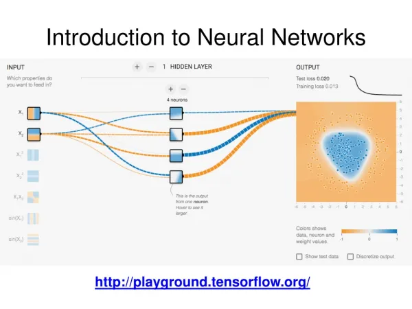
26. Artificial Neural Network (ANN) • Made of artificial neurons, each of which • Sums inputs xi from other neurons • Compares sum to threshold • Sends signal to other neurons if above threshold • Synapses have weights • Model relative ion collections • Model efficacy (strength) of synapse

27. Artificial Neuron Nonlinear firing function . . .

28. First Generation: 1957 - 1969 • Best Understood in terms of Classifiers • Partition a data space into regions containing data points of the same classification. • The regions are predictions of the classification of new data points.

29. Simple Perceptron Model • Given 2 classes – Reference and Sample • Firing function (activation function) has only two values, 0 or 1. • “Learning” is by incremental updating of weights using a linear learning rule w1 w2 wn

30. Perceptron Limitations • Cannot Do XOR (1969, Minsky and Papert) • Data must be linearly separable • 1970’s: ANN’s “Wilderness Experience” – only a handful working and very “un-neuron-like”

31. Support Vector Machine: Perceptron on a Feature Space • Data is projected into a high-dimensional Feature Space, separated with a hyperplane • Choice of Feature Space (kernel) is key. • Predictions based on location of hyperplane

32. Second Generation: 1981 - Soon • Big Ideas from other Fields • J. J. Hopfield compares neural networks to Ising Spin Glass models. Uses statistical Mechanics to prove that ANN’s minimize a total energy functional. • Cognitive Psychology provides new insights into how neural networks learn. • Big Ideas from Math • Kolmogorov’s Theorem AND

33. Firing Functions are Sigmoidal

34. 3 Layer Neural Network The output layer may consist of a single neuron Output Input Hidden (is usually much larger)

35. Multilayer Network . . . . . .

36. Hilbert’s Thirteenth Problem • Original: “Are there continuous functions of 3 variables that are not representable by a superposition of composition of functions of 2 variables?” • Modern: Can a continuous function of n variables on a bounded domain of n-space be written as sums of compositions of functions of 1 variable?

37. Kolmogorov’s Theorem Modified Version: Any continuous function f of n variables can be written where only h and w’s depend on f (That is, the g’s are fixed)

38. Cybenko (1989) Let s be any continuous sigmoidal function, and let x = (x1,…,xn). If f is absolutely integrable over the n-dimensional unit cube, then for all e>0, there exists a (possibly very large ) integer N and vectors w1,…,wN such that where a1,…,aN and q1,…,qN are fixed parameters.

39. Multilayer Network (MLP’s) . . . . . .

40. ANN as a Universal Classifier • Designs a function f : Data -> Classes • Example: f ( Red ) = 1, f ( Blue) = 0 • Support of f defines the regions • Data is used to train (i.e., design ) function f supp(f)

41. Example – Predicting Trees that are or are not RNA-like RNA Like NotRNA Like • Construct Graphical Invariants • Train ANN using known RNA-trees • Predict the others

42. This tiny 3-Dimensional Artificial Neural Network, modeled after neural networks in the human brain, is helping machines better visualize their surroundings. 2nd Generation: Phenomenal Success • Data Mining of Micro-array data • Stock and commodities trading: ANN’s are an important part of “computerized trading” • Post office mail sorting

43. The Mars Rovers • ANN decides between “rough” and “smooth” • “rough” and “smooth” are ambiguous • Learningvia many“examples” And a neural network can lose up to 10% of its neurons without significant loss in performance!

44. Overfitting may Produce Isolated Regions ANN Limitations • Overfitting: e.g, if Training Set is “unbalanced” • Mislabeled data can lead to slow (or no) convergence or incorrect results. • Hard Margins: No “fuzzing” of the boundary

45. Problems on the Horizon • Limitations are becoming very limiting • Trained networks often are poor learners (and self-learners are hard to train) • In real neural networks, more neurons imply better networks (not so in ANNs ). • Temporal data is problematic – ANN’s have no concept or a poor concept of time • “Hybridized ANN’s” becoming the rule • SVM’s probably the tool of choice at present • SOFM’s, Fuzzy ANN’s, Connectionism

46. Third Generation: 1997 - • Back to Bio: Spiking Neural Networks (SNN) • Asynchronous, action-potential driven ANN’s have been around for some time. • SNN’s show “promise” but results beyond current ANN’s have been elusive • Simulating actual HH equations (neuromimetic) has to date not been enough • Time is both a promise and a curse • A Possible Approach: Use current dendritic models to modify existing ANN’s.

47. ANN’s with Multiple Time Scales • SNN that reduces to ANN & preserves Kolmogorov Thm • The solution to the equiv cylinder with hotspots is where Ij is the restriction of V to jth “hot spot”. • Equivalent Artificial Neuron:

48. Incorporating MultiExponentials • G(0,x,t) is often a multi-exponential decay. • In terms of time constants tk • wjk are synaptic “weights” • tk from electrotonic and morphometric data • Rate of taper, Length of dendrites • Branching, capacitance, resistance

49. Approximation and Simplification • If xj(u) approx 1 or xj(u) approx 0, then • A Special Case (k is a constant) • t = 0 yields the standard Neural Net Model • Standard Neural Net as initial Steady State • Modify with time-dependent transient

50. Artificial Neuron wij, pij = synaptic weights Nonlinear firing function wi1, pi1 . . . win, pin