Download

1 / 41
410 likes | 514 Views
This lecture from CS 477/677, taught by Instructor Monica Nicolescu, delves into essential graph algorithms, focusing on Breadth-First Search (BFS) and Strongly Connected Components (SCC). Students learn to process graphs, determine distances from a source vertex, and carry out depth-first searches. Key concepts like topological sorting, graph transposes, and the relationship between graph structure and connected components are explored. The process of identifying SCCs through depth-first search techniques is examined in detail, providing foundational insights into graph theory's applications.

E N D
Analysis of AlgorithmsCS 477/677 Instructor: Monica Nicolescu Lecture 22
Breadth-First Search (BFS) • Input: • A graph G = (V, E) (directed or undirected) • A source vertex s V • Goal: • Explore the edges of G to “discover” every vertex reachable from s, taking the ones closest to s first • Output: • d[v] = distance (smallest # of edges) from s to v, for all v V • A “breadth-first tree” rooted at s that contains all reachable vertices CS 477/677 - Lecture 22
2 1 3 5 4 Depth-First Search • Input: • G = (V, E) (No source vertex given!) • Goal: • Explore the edges of G to “discover” every vertex in V starting at the most current visited node • Search may be repeated from multiple sources • Output: • 2 timestamps on each vertex: • d[v] = discovery time • f[v] = finishing time (done with examining v’s adjacency list) • Depth-first forest CS 477/677 - Lecture 22
socks undershorts pants shoes watch shirt belt tie jacket Topological Sort undershorts socks Topological sort: - a linear order of vertices such that if there exists an edge (u, v), then u appears before v in the ordering - all directed edges go from left to right. pants shoes shirt belt watch tie jacket CS 477/677 - Lecture 22
Strongly Connected Components Given directed graph G = (V, E): A strongly connected component (SCC) of G is a maximal set of vertices C V such that for every pair of vertices u, v C, we have both u v and v u. CS 477/677 - Lecture 22
2 2 1 1 3 3 5 5 4 4 The Transpose of a Graph • GT = transposeof G • GT is G with all edges reversed • GT = (V, ET), ET = {(u, v) : (v, u) E} • If using adjacency lists: we can create GT in (|V| + |E|) time CS 477/677 - Lecture 22
2 2 1 1 3 3 5 5 4 4 Finding the SCC • Observation: G and GT have the same SCC’s • u and v are reachable from each other in G they are reachable from each other in GT • Idea for computing the SCC of a graph G = (V, E): • Make two depth first searches: one on G and one on GT CS 477/677 - Lecture 22
STRONGLY-CONNECTED-COMPONENTS(G) • call DFS(G) to compute finishing times f[u] for each vertex u • compute GT • call DFS(GT), but in the main loop of DFS, consider vertices in order of decreasing f[u] (as computed in first DFS) • output the vertices in each tree of the depth-first forest formed in second DFS as a separate SCC CS 477/677 - Lecture 22
a b c d e f g h a b c d e f g h Example DFS on the initial graph G 13/ 14 11/ 16 1/ 10 8/ 9 b 16 e 15 a 14 c 10 d 9 g 7 h 6 f 4 3/ 4 2/ 7 5/ 6 12/ 15 • DFS on GT: • start at b: visit a, e • start at c: visit d • start at g: visit f • start at h Strongly connected components: C1 = {a, b, e}, C2 = {c, d}, C3 = {f, g}, C4 = {h} CS 477/677 - Lecture 22
c d a b c d a b e f g h e f g h Component Graph • The component graph GSCC = (VSCC, ESCC): • VSCC = {v1, v2, …, vk}, where vi corresponds to each strongly connected component Ci • There is an edge (vi, vj) ESCC if G contains a directed edge (x, y) for some x Ci and y Cj • The component graph is a DAG CS 477/677 - Lecture 22
Lemma 1 Let C and C’ be distinct SCC’s in G Let u, v C, and u’, v’ C’ Suppose there is a path u u’ in G Then there cannot also be a path v’ v in G. Proof • Suppose there is a path v’ v • There exists u u’ v’ • There exists v’ v u • u and v’ are reachable from each other, so they are not in separate SCC’s: contradiction! C’ C u u’ v v’ CS 477/677 - Lecture 22
d(C2) =1 d(C1) =11 f(C2) =10 f(C1) =16 d(C4) d(C3) =5 =2 f(C4) f(C3) =6 =7 Notations • Extend notation for d (starting time) and f (finishing time) to sets of vertices U V: • d(U) = minuU { d[u] } (earliest discovery time) • f(U) = maxuU { f[u] } (latest finishing time) C1 C2 a b c d 13/ 14 11/ 16 1/ 10 8/ 9 3/ 4 2/ 7 5/ 6 12/ 15 e f g h C4 C3 CS 477/677 - Lecture 22
d(C2) =1 d(C1) =11 f(C2) =10 f(C1) =16 d(C4) d(C3) =5 =2 f(C4) f(C3) =6 =7 Lemma 2 • Let C and C’ be distinct SCCs in a directed graph G = (V, E). If there is an edge (u, v) E, where u C and v C’ then f(C) > f(C’). • Consider C1 and C2, connected by edge (b, c) C1 C2 a b c d 13/ 14 11/ 16 1/ 10 8/ 9 3/ 4 2/ 7 5/ 6 12/ 15 e f g h C4 C3 CS 477/677 - Lecture 22
a b c d e f g h Corollary (alternative formulation) f(C) < f(C’) • Each edge in GT that goes between different components goes from a component with an earlier finish time (in the DFS) to one with a later finish time C1 = C’ C2 = C C4 C3 CS 477/677 - Lecture 22
a b c d b 16 e 15 a 14 c 10 d 9 g 7 h 6 f 4 e f g h Why does SCC Work? • When we do the second DFS, on GT, we start with a node in a component C such that f(C) is maximum (b, in our case) • We start from b and visit all vertices in C1 • From corollary: f(C) > f(C’) for all C C’ there are no edges from C to any other SCCs in GT DFS will visit only vertices in C1 The depth-first tree rooted at b contains exactly the vertices of C1 C1 C2 C3 C4 CS 477/677 - Lecture 22
a b c d b 16 e 15 a 14 c 10 d 9 g 7 h 6 f 4 e f g h Why does SCC Work? (cont.) • The next root chosen in the second DFS is in SCC C2 such that f(C) is maximum over all SCC’s other than C1 • DFS visits all vertices in C2 • the only edges out of C2 go to C1, which we’ve already visited The only tree edges will be to vertices in C2 • Each time we choose a new root it can reach only: • vertices in its own component • vertices in components already visited C1 C2 C3 C4 CS 477/677 - Lecture 22
8 7 b c d 9 4 2 a e i 11 14 4 6 7 8 10 h g f 2 1 Minimum Spanning Trees Problem • A town has a set of houses and a set of roads • A road connects 2 and only 2 houses • A road connecting houses u and v has a repair cost w(u, v) Goal: Repair enough (and no more) roads such that: • Everyone stays connected: can reach every house from all other houses, and • Total repair cost is minimum CS 477/677 - Lecture 22
8 7 b c d 9 4 2 a e i 11 14 4 6 7 8 10 h g f 2 1 Minimum Spanning Trees • A connected, undirected graph: • Vertices = houses, Edges = roads • A weight w(u, v) on each edge (u, v) E Find T E such that: • T connects all vertices • w(T) = Σ(u,v)T w(u, v) is minimized CS 477/677 - Lecture 22
8 7 b c d 9 4 2 a e i 11 14 4 6 7 8 10 h g f 2 1 Minimum Spanning Trees • T forms a tree = spanning tree • A spanning tree whose weight is minimum over all spanning trees is called a minimum spanning tree, or MST. CS 477/677 - Lecture 22
8 7 b c d 9 4 2 a e i 11 14 4 6 7 8 10 h g f 2 1 Properties of Minimum Spanning Trees • Minimum spanning trees are not unique • Can replace (b, c) with (a, h) to obtain a different spanning tree with the same cost • MST have no cycles • We can take out an edge of a cycle, and still have all vertices connected while reducing the cost • # of edges in a MST: • |V| - 1 CS 477/677 - Lecture 22
8 7 b c d 9 4 2 a e i 11 14 4 6 7 8 10 h g f 2 1 Growing a MST Minimum-spanning-tree problem: find a MST for a connected, undirected graph, with a weight function associated with its edges A generic solution: • Build a set A of edges (initially empty) • Incrementally add edges to A such that they would belong to a MST • An edge (u, v) is safe for A if and only if A {(u, v)} is also a subset of some MST We will add only safe edges CS 477/677 - Lecture 22
8 7 b c d 9 4 2 a e i 11 14 4 6 7 8 10 h g f 2 1 GENERIC-MST • A ← • while A is not a spanning tree • do find an edge (u, v) that is safe for A • A ← A {(u, v)} • return A • How do we find safe edges? CS 477/677 - Lecture 22
8 V - S 7 b c d 9 4 2 a e i 11 14 4 6 7 8 10 S h g f 2 1 Finding Safe Edges • Let’s look at edge (h, g) • Is it safe for A initially? • Later on: • Let S V be any set of vertices that includes h but not g (so that g is in V - S) • In any MST, there has to be one edge (at least) that connects S with V - S • Why not choose the edge with minimum weight (h,g)? CS 477/677 - Lecture 22
8 7 b c d 9 4 2 a e i 11 14 4 6 7 8 10 h g f 2 1 Definitions • A cut (S, V - S) is a partition of vertices into disjoint sets S and V - S • An edge crosses the cut (S, V - S) if one endpoint is in S and the other in V – S • A cut respects a set A of edges no edge in A crosses the cut • An edge is a light edge crossing a cut its weight is minimum over all edges crossing the cut • For a given cut, there can be several light edges crossing it S S V- S V- S CS 477/677 - Lecture 22
S u v V - S Theorem • Let A be a subset of some MST, (S, V - S) be a cut that respects A, and (u, v) be a light edge crossing (S, V - S). Then (u, v) is safe for A. Proof: • Let T be a MST that includes A • Edges in A are shaded • Assume T does not include the edge (u, v) • Idea: construct another MST T’ that includes A {(u, v)} CS 477/677 - Lecture 22
Discussion In GENERIC-MST: • A is a forest containing connected components • Initially, each component is a single vertex • Any safe edge merges two of these components into one • Each component is a tree • Since an MST has exactly |V| - 1 edges: after iterating |V| - 1 times, we have only one component CS 477/677 - Lecture 22
We would add edge (c, f) 8 7 b c d 9 4 2 a e i 11 14 4 6 7 8 10 h g f 2 1 The Algorithm of Kruskal • Start with each vertex being its own component • Repeatedly merge two components into one by choosing the light edge that connects them • Scan the set of edges in monotonically increasing order by weight • Uses a disjoint-set data structure to determine whether an edge connects vertices in different components CS 477/677 - Lecture 22
Operations on Disjoint Data Sets • MAKE-SET(u) – creates a new set whose only member is u • FIND-SET(u) – returns a representative element from the set that contains u • May be any of the elements of the set that has a particular property • E.g.: Su = {r, s, t, u}, the property may be that the element is the first one alphabetically FIND-SET(u) = r FIND-SET(s) = r • FIND-SET has to return the same value for a given set CS 477/677 - Lecture 22
Operations on Disjoint Data Sets • UNION(u, v) – unites the dynamic sets that contain u and v, say Su and Sv • E.g.: Su = {r, s, t, u}, Sv = {v, x, y} UNION (u, v) = {r, s, t, u, v, x, y} CS 477/677 - Lecture 22
KRUSKAL(V, E, w) • A ← • for each vertex v V • do MAKE-SET(v) • sort E into increasing order by weight w • for each (u, v) taken from the sorted list • do if FIND-SET(u) FIND-SET(v) • then A ← A {(u, v)} • UNION(u, v) • return A Running time: O(|E| lg|V|) – dependent on the implementation of the disjoint-set data structure CS 477/677 - Lecture 22
8 7 b c d 9 4 2 a e i 11 14 4 6 7 8 10 h g f 2 1 Example • Add (h, g) • Add (c, i) • Add (g, f) • Add (a, b) • Add (c, f) • Ignore (i, g) • Add (c, d) • Ignore (i, h) • Add (a, h) • Ignore (b, c) • Add (d, e) • Ignore (e, f) • Ignore (b, h) • Ignore (d, f) {g, h}, {a}, {b}, {c}, {d}, {e}, {f}, {i} {g, h}, {c, i}, {a}, {b}, {d}, {e}, {f} {g, h, f}, {c, i}, {a}, {b}, {d}, {e} {g, h, f}, {c, i}, {a, b}, {d}, {e} {g, h, f, c, i}, {a, b}, {d}, {e} {g, h, f, c, i}, {a, b}, {d}, {e} {g, h, f, c, i, d}, {a, b}, {e} {g, h, f, c, i, d}, {a, b}, {e} {g, h, f, c, i, d, a, b}, {e} {g, h, f, c, i, d, a, b}, {e} {g, h, f, c, i, d, a, b, e} {g, h, f, c, i, d, a, b, e} {g, h, f, c, i, d, a, b, e} {g, h, f, c, i, d, a, b, e} 1: (h, g) 2: (c, i), (g, f) 4: (a, b), (c, f) 6: (i, g) 7: (c, d), (i, h) 8: (a, h), (b, c) 9: (d, e) 10: (e, f) 11: (b, h) 14: (d, f) {a}, {b}, {c}, {d}, {e}, {f}, {g}, {h},{i} CS 477/677 - Lecture 22
8 7 b c d 9 4 2 a e i 11 14 4 6 7 8 10 h g f 2 1 The Algorithm of Prim • The edges in set A always form a single tree • Starts from an arbitrary “root”: VA = {a} • At each step: • Find a light edge crossing cut (VA, V - VA) • Add this edge to A • Repeat until the tree spans all vertices • Greedy strategy • At each step the edge added contributes the minimum amount possible to the weight of the tree CS 477/677 - Lecture 22
8 7 b c d 9 4 2 a e i 11 14 4 6 7 8 10 h g f 2 1 How to Find Light Edges Quickly? Use a priority queue Q: • Contains all vertices not yet included in the tree (V – VA) • V = {a}, Q = {b, h, c, d, e, f, g, i} • With each vertex v we associate a key: key[v] = minimum weight of any edge (u, v) connecting v to a vertex in the tree • Key of v is if v is not adjacent to any vertices in VA • After adding a new node to VA we update the weights of all the nodes adjacent to it • We added node a key[b] = 4, key[h] = 8 CS 477/677 - Lecture 22
8 7 b c d 9 4 2 a e i 11 14 4 6 7 8 10 h g f 2 1 PRIM(V, E, w, r) • Q ← • for each u V • do key[u] ← ∞ • π[u] ← NIL • INSERT(Q, u) • DECREASE-KEY(Q, r, 0) • while Q • do u ← EXTRACT-MIN(Q) • for each vAdj[u] • do if v Q and w(u, v) < key[v] • then π[v] ← u • DECREASE-KEY(Q, v, w(u, v)) 0 0 Q = {a, b, c, d, e, f, g, h, i} VA = Extract-MIN(Q) a CS 477/677 - Lecture 22
4 8 8 8 7 7 b b c c d d 9 9 4 4 2 2 a a e e i i 11 11 14 14 4 4 6 6 7 7 8 8 10 10 h h g g f f 2 2 1 1 Example 0 Q = {a, b, c, d, e, f, g, h, i} VA = Extract-MIN(Q) a key [b] = 4 [b] = a key [h] = 8 [h] = a 4 8 Q = {b, c, d, e, f, g, h, i} VA = {a} Extract-MIN(Q) b CS 477/677 - Lecture 22
4 8 8 8 7 7 b b c c d d 8 4 9 9 4 4 2 2 a a e e i i 11 11 14 14 4 4 6 6 7 7 8 8 10 10 h h g g f f 2 2 1 1 8 Example key [c] = 8 [c] = b key [h] = 8 [h] = a - unchanged 8 8 Q = {c, d, e, f, g, h, i} VA = {a, b} Extract-MIN(Q) c 8 key [d] = 7 [d] = c key [f] = 4 [f] = c key [i] = 2 [i] = c 7 4 8 2 Q = {d, e, f, g, h, i} VA = {a, b, c} Extract-MIN(Q) i 7 2 4 CS 477/677 - Lecture 22
8 8 7 7 b b c c d d 8 4 7 8 4 7 9 9 4 4 2 2 a a e e i i 11 11 14 14 4 4 2 2 6 6 7 7 8 8 10 10 h h g g f f 2 2 1 1 4 8 4 6 7 Example key [h] = 7 [h] = i key [g] = 6 [g] = i 7 4 6 7 Q = {d, e, f, g, h} VA = {a, b, c, i} Extract-MIN(Q) f key [g] = 2 [g] = f key [d] = 7 [d] = c unchanged key [e] = 10 [e] = f 7 10 2 7 Q = {d, e, g, h} VA = {a, b, c, i, f} Extract-MIN(Q) g 6 7 10 2 CS 477/677 - Lecture 22
8 8 7 7 b b c c d d 8 8 4 4 7 7 9 9 4 4 2 2 a a e e i i 11 11 14 14 4 4 10 10 2 2 6 6 7 7 8 8 10 10 h h g g f f 2 2 1 1 4 4 2 2 7 1 Example key [h] = 1 [h] = g 7 10 1 Q = {d, e, h} VA = {a, b, c, i, f, g} Extract-MIN(Q) h 7 10 Q = {d, e} VA = {a, b, c, i, f, g, h} Extract-MIN(Q) d 1 CS 477/677 - Lecture 22
8 7 b c d 8 4 7 9 4 2 a e i 11 14 4 10 2 6 7 8 10 h g f 2 1 4 2 1 Example key [e] = 9 [e] = d 9 Q = {e} VA = {a, b, c, i, f, g, h, d} Extract-MIN(Q) e Q = VA = {a, b, c, i, f, g, h, d, e} 9 CS 477/677 - Lecture 22
PRIM(V, E, w, r) Total time: O(VlgV + ElgV) = O(ElgV) • Q ← • for each u V • do key[u] ← ∞ • π[u] ← NIL • INSERT(Q, u) • DECREASE-KEY(Q, r, 0) ► key[r] ← 0 • while Q • do u ← EXTRACT-MIN(Q) • for each vAdj[u] • do if v Q and w(u, v) < key[v] • then π[v] ← u • DECREASE-KEY(Q, v, w(u, v)) O(V) if Q is implemented as a min-heap Min-heap operations: O(VlgV) Executed V times Takes O(lgV) Executed O(E) times O(ElgV) Constant Takes O(lgV) CS 477/677 - Lecture 22
Readings • Chapter 23 CS 477/677 - Lecture 22