Download
1 / 39
390 likes | 414 Views
Explore search structures and hashing techniques for implementing a dynamic dictionary. Learn about different implementations, collision resolution methods, and the use of hash functions.

E N D
Lecture 10:Search Structures and Hashing Shang-Hua Teng
Dictionary/Table Keys Operation supported: search Given a student ID find the record (entry)
Keys Entry Data Format
What if student ID is 9-digit social security number • Well, we can still sort by the ids and apply binary search. • If we have n students, we need O(n) space • And O(log n) search time
What if new students come and current students leave • Dynamic dictionary • Yellow page update once in a while • Which is not truly dynamic • Operations to support • Insert: add a new (key, entry) pair • Delete: remove a (key, entry) pair from the dictionary • Search: Given a key, find if it is in the dictionary, and if it is , return the data entry associated with the key
How should we implement a dynamic dictionary? • How often are entries inserted and removed? • How many of the possible key values are likely to be used? • What is the likely pattern of searching for keys?
key entry “Smith” “Smith”, “124 Hawkers Lane”, “9675846” “Yao” “Yao”, “1 Apple Crescent”, “0044 1970 622455” (Key,Entry) pair • For searching purposes, it is best to store the key and the entry separately (even though the key’s value may be inside the entry) (key,entry)
Implementation 1:unsorted sequential array • An array in which (key,entry)-pair are stored consecutively in any order • insert: add to the back of array; O(1) • search: search through the keys one at a time, potentially all of the keys; O(n) • remove: find + replace removed node with last node; O(n) key entry 0 1 2 3 … and so on
Implementation 2:sorted sequential array • An array in which (key,entry) pair are stored consecutively, sorted by key • insert: add in sorted order; O(n) • find: binary search; O(log n) • remove: find, remove node and shuffle down; O(n) key entry 0 1 2 3 … and so on
Implementation 3:linked list (unsorted or sorted) • (key,entry) pairs are again stored consecutively • insert: add to front; O(1)or O(n) for a sorted list • find: search through potentially all the keys, one at a time; O(n)still O(n) for a sorted list • remove: find, remove using pointer alterations; O(n) key entry and so on
Direct Addressing • Suppose: • The range of keys is 0..m-1 (Universe) • Keys are distinct • The idea: • Set up an array T[0..m-1] in which • T[i] = x if x T and key[x] = i • T[i] = NULL otherwise
0 / entry 1 1 2 / 3 / 7 4 / 1 5 5 5 6 / 7 7 Direct-address Table • Direct addressing is a simple technique that works well when the universe of keys is small. Assuming each key corresponds to a unique slot. Direct-Address-Search(T,k) return T[k] Direct-Address-Insert(T,x) return T[key[x]] x Direct-Address-Delete(T,x) return T[key[x]] Nil O(1) time for all operations
The Problem With Direct Addressing • Direct addressing works well when the range m of keys is relatively small • But what if the keys are 32-bit integers? • Problem 1: direct-address table will have 232 entries, more than 4 billion • Problem 2: even if memory is not an issue, the time to initialize the elements to NULL may be • Solution: map keys to smaller range 0..m-1 • This mapping is called a hash function
T 0 U(universe of keys) h(k1) k1 h(k4) k4 K(actualkeys) k5 h(k2) = h(k5) k2 h(k3) k3 m - 1 Hash function • A hash function determines the slot of the hash table where the key is placed. • Previous example the hash function is the identity function • We say that a record with key k hashes into slot h(k)
Next Problem • collision T 0 U(universe of keys) h(k1) k1 h(k4) k4 K(actualkeys) k5 h(k2) = h(k5) k2 h(k3) k3 m - 1
Pigeonhole Principle Parque de las Palomas San Juan, Puerto Rico
Resolving Collisions • How can we solve the problem of collisions? • Solution 1: chaining • Solution 2: open addressing
k5 k2 —— k6 —— Chaining • Chaining puts elements that hash to the same slot in a linked list: T —— U(universe of keys) k4 k1 —— —— k1 —— k4 K(actualkeys) k5 —— k7 k7 —— k3 k2 k3 —— k8 k6 k8 ——
Chaining (insert at the head) T —— U(universe of keys) k1 —— —— k1 —— k4 K(actualkeys) k5 —— k7 —— —— k3 k2 k8 —— k6 —— ——
Chaining (insert at the head) T —— U(universe of keys) k1 —— —— k1 —— k4 K(actualkeys) k5 —— k7 k2 —— —— k3 k2 k3 —— k8 k6 —— ——
k4 k1 —— Chaining (insert at the head) T —— U(universe of keys) k1 —— —— k1 —— k4 K(actualkeys) k5 —— k7 k2 —— —— k3 k2 k3 —— k8 k6 —— ——
k4 k1 —— k5 k2 —— k6 —— Chaining (insert at the head) T —— U(universe of keys) k1 —— —— k1 —— k4 K(actualkeys) k5 —— k7 k2 —— —— k3 k2 k3 —— k8 k6 ——
k5 k2 —— k6 —— Chaining (Insert to the head) T —— U(universe of keys) k4 k1 —— —— k1 —— k4 K(actualkeys) k5 —— k7 k7 —— k3 k2 k3 —— k8 k6 k8 ——
Operations Direct-Hash-Search(T,k) Search for an element with key k in list T[h(k)] (running time is proportional to length of the list) Direct-Hash-Insert(T,x) (worst case O(1)) Insert x at the head of the list T[h(key[x])] Direct-Hash-Delete(T,x) Delete x from the list T[h(key[x])] (For singly linked list we might need to find the predecessor first. So the complexity is just like that of search)
Analysis of hashing with chaining • Given a hash table with m slots and n elements • The load factor = n/m • The worst case behavior is when all n elements hash into the same location ((n) for searching) • The average performance depends on how well the hash function distributes elements • Assumption: simple uniform hashing: Any element is equally likely to hash into any of the m slot • For any key h(k) can be computed in O(1) • Two cases for a search: • The search is unsuccessful • The search is successful
Unsuccessful search Theorem 11.1 : In a hash table in which collisions are resolved by chaining, an unsuccessful search takes (1+ ), on the average, under the assumption of simple uniform hashing. Proof: • Simple uniform hashing any key k is equally likely to hash into any of the m slots. • The average time to search for a given key k is the time it takes to search a given slot. • The average length of each slot is = n/m: the load factor. • The time it takes to compute h(k) is O(1). • Total time is (1+).
Successful Search Theorem 11.2 : In a hash table in which collisions are resolved by chaining, a successful search takes (1+ /2 ), under the assumption of simple uniform hashing. Proof: • Simple uniform hashing any key k is equally likely to hash into any of the m slots. • Note Chained-Hash-Insert inserts a new element in the front of the list • The expected number of elements visited during the search is 1 more than the number of elements of the list after the element is inserted
Successful Search • Take the average over the n elements • (i 1)/m is the expected length of the list to which i was added. The expected length of each list increases as more elements are added. (1) (2) (3)
Analysis of Chaining • Assume simple uniform hashing: each key in table is equally likely to be hashed to any slot • Given n keys and m slots in the table, the load factor = n/m = average # keys per slot • What will be the average cost of an unsuccessful search for a key?O(1+) • What will be the average cost of a successful search?O(1 +/2) = O(1 + )
Choosing A Hash Function • Choosing the hash function well is crucial • Bad hash function puts all elements in same slot • A good hash function: • Should distribute keys uniformly into slots • Should not depend on patterns in the data • Three popular methods: • Division method • Multiplication method • Universal hashing
The Division Method • h(k) = k mod m • In words: hash k into a table with m slots using the slot given by the remainder of k divided by m • Elements with adjacent keys hashed to different slots: good • If keys bear relation to m: bad • In Practice: pick table size m = prime number not too close to a power of 2 (or 10)
The Multiplication Method • For a constant A, 0 < A < 1: • h(k) = m (kA - kA) • In practice: • Choose m = 2P • Choose A not too close to 0 or 1 • Knuth: Good choice for A = (5 - 1)/2 Fractional part of kA
Universal Hashing • When attempting to foil an malicious adversary, randomize the algorithm • Universal hashing: pick a hash function randomly when the algorithm begins • Guarantees good performance on average, no matter what keys adversary chooses • Need a family of hash functions to choose from • Think of quick-sort
Universal Hashing • Let Gbe a (finite) collection of hash functions • …that map a given universe U of keys… • …into the range {0, 1, …, m - 1}. • Gis said to be universal if: • for each pair of distinct keys x, y U,the number of hash functions h Gfor which h(x) = h(y) is |G|/m • In other words: • With a random hash function from G the chance of a collision between x and y is exactly 1/m (x y)
Universal Hashing • Theorem 11.3: • Choose h from a universal family of hash functions • Hash n keys into a table of m slots, nm • Then the expected number of collisions involving a particular key x is less than 1 • Proof: • For each pair of keys y, z, let cyx= 1 if y and z collide, 0 otherwise • E[cyz] = 1/m (by definition) • Let Cx be total number of collisions involving key x • Since nm, we have E[Cx] < 1
A Universal Hash Function • Choose table size m to be prime • Decompose key x into r+1 bytes, so that x = {x0, x1, …, xr} • Only requirement is that max value of byte < m • Let a = {a0, a1, …, ar} denote a sequence of r+1 elements chosen randomly from {0, 1, …, m - 1} • Define corresponding hash function ha G: • With this definition, Ghas mr+1 members
A Universal Hash Function • Gis a universal collection of hash functions (Theorem 11.5) • How to use: • Pick r based on m and the range of keys in U • Pick a hash function by (randomly) picking the a’s • Use that hash function on all keys
Example • Let m = 5, and the size of each string is 2 bits (binary). Note the maximum value of a string is 3 and m = 5 • a = 1,3, chosen at random from 0,1,2,3,4 • Example for x = 4 = 01,00 (note r = 1) • ha(4) = 1 (01) + 3 (00) = 1
Open Addressing • Basic idea (details in Section 12.4): • To insert: if slot is full, try another slot, …, until an open slot is found (probing) • To search, follow same sequence of probes as would be used when inserting the element • If reach element with correct key, return it • If reach a NULL pointer, element is not in table • Good for fixed sets (adding but no deletion) • Table needn’t be much bigger than n