Download
1 / 17
170 likes | 318 Views
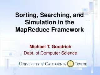
Sorting, Searching, and Simulation in the MapReduce Framework . Michael T. Goodrich Dept. of Computer Science. MapReduce. A framework for designing computations for large clusters of computers. Decouples location from data and computation.

E N D
Sorting, Searching, and Simulation in the MapReduce Framework Michael T. Goodrich Dept. of Computer Science
MapReduce • A framework for designing computations for large clusters of computers. • Decouples location from data and computation Image from taken from Yahoo! Hadoop Presentation: Part 2, OSCON 2007.
Map-Shuffle-Reduce • Map: • (k,v) -> [(k1,v1),(k2,v2),…] • must depend only on this one pair, (k,v) • Shuffle: • For each key k used in the first coordinate of a pair, collect all pairs with k as first coordinate • [(k,v1),(k,v2),…] • Reduce: • For each list, [(k,v1),(k,v2),…]: • Perform a sequential computation to produce a set of pairs, [(k’1,v’1),(k’2,v’2),…] • Pairs from this reduce step can be output or used in another map-shuffle-reduce cycle. Image from http://www.wvculture.org/shpo/es/graphics/6-sorting%20shell.jpg
A Simple Example • Count number of occurrences of each word in a large document or corpus • Map: (word,null) -> (word,1) • Shuffle: groups occurrences of each word • Reduce: count number of 1’s in each list • This has one round of computation, but can take a long time (e.g., 7% of all English words are “the”). Image from http://peterpappas.blogs.com/copy_paste/2009/01/build-literacy-skills-with-wordle.html
Evaluating MapReduce Algorithms • If map/reduce time is dominated by a buffer-size, B, parallelism is increased. • So time is dominated by number of rounds and message complexity • Eliminates false efficiency of the trivial one-round algorithm • similar approaches were used by • [Feldman et al., 08], who choose B=polylog(n) • [Karloff et al., 10], who choose B=n1-e • We choose B=n1/k, for a given integer parameter, k>0, to allow for a spectrum of possible buffer sizes, e.g., k=2, 3, or 4 would be natural for real-world problem instances
Our Results • Label a set of inputs from 1..N in O(k) rounds • Simulate any bulk-synchronous parallel (BSP) algorithm with constant overhead • extends constant-overhead EREW PRAM simulation of [Karloff et al., 10] • Simulate any CRCW PRAM algorithm with an overhead of O(k) per PRAM step • Applications: sorting, 2-d/3-d convex hulls, fixed-d linear programming in O(k) rounds • Perform multisearching of a tree of size n with n searches
Invisible B-Trees • Define a B-tree labeling, (L,i), where L is a level and i is an index. • Each node knows its parent-node label and its children labels • Perform a top-down or bottom-up computation in such a tree, automatically ignoring missing nodes. Image from http://svn.apache.org/repos/asf/xml/xindice/trunk/src/documentation/resources/images/
Invisible B-Trees • Allows for tree-based computations that utilize only the necessary nodes. 1,1 2,1 2,2 2,3 3,1 3,2 3,3 3,4 3,5 3,6 3,7 3,8 3,9 4,27 4,2 4,6 4,8 4,9 4,14 4,20 4,1 4,3 4,7 4,26 4,5 4,13 4,15 4,19 4,21 4,25 4,4
Index-Labeling the Input • B-arydistribute-and-combine: • Assign each pair a random value from 1 to N3 • Apply invisible B-tree technique to perform a bottom-up sum (with each tuple worth 1) • Perform a top-down prefix sum computation • Now the pairs are numbered 1 to N. • Takes O(logB N) = O(k) rounds. Image from http://www.nevron.com/gallery/FullGalleries/diagram/symmetrical/images/binaryTree.png
BSP Simulation • Each super-step involves sending/receiving B messages. • To simulate: • Create a tuple for each memory cell and processor • Map each message to the destination processor label, P. • Reduce by performing one step of processor P, outputting the messages for next round. • Theorem: Given a BSP algorithm A that runs in T super-steps with a total memory size N using P < N processors, we can simulate A using T rounds and message complexity O(TM) in the memory-bound MapReduce framework with reducer buffer size bounded by B = N/P and total memory size M. • Some implications…
MapReduce Sorting • Given the optimal BSP algorithm of [Goodrich, 99], we can sort N values in the MapReduce framework in O(k) rounds and O(kN) message complexity. Image from http://www.hatfulofhollow.com/posts/code/visualisingsorting/
MapReduce Convex Hulls • Given BSP algorithms of [Goodrich, 97], we can do 2-d and 3- convex hulls in O(k) rounds, w.h.p., with message complexity O(kN). Image from http://www.algorithmist.com/index.php/Monotone_Chain_Convex_Hull
CRCW PRAM Simulation • Create tuples for memory cells and processors. • For each memory access, use an invisible B-tree to map read/write requests to the memory cells and back to the processors. • Allows us to simulate even the most powerful version of the CRCW PRAM, where writes are combined according to an associative function • Theorem: Given an algorithm A in the CRCW PRAM model, with write conflicts resolved according to a commutative semigroup function, f, such that A runs in T steps using P processors and N memory cells, we can simulate A in the memory-bound MapReduce framework in O(kT) rounds and O(kT(N + P)) message complexity, where k=O(logB P). Image from http://sky.geocities.jp/enokiec/enokiepisode/KeypunchSorting.jpg
Fixed-d Linear Programming • [Alon and Meggido, 94] give a constant-time CRCW PRAM algorithm for fixed-d linear programming w.h.p. • This gives us a MapReduce algorithm running in time O(k) w.h.p. Image from http://people.richland.edu/james/lecture/m116/systems/linear.html
Multisearching • Given: a binary tree T of size n and a set Q of n queries to perform on T. Q={q1,q2,…,qn} • [Goodrich 97] gives a BSP solution, but it would require O(n log2 n) message complexity to simulate it in the MapReduce framework. T:
Pipelined Multisearching • Break Q into k random groups of size n/k each. • Sample from Q1 to get an estimate of the query distribution. • Build the circuit of [Goodrich 97] for Q1. • Pipeline all the queries through this circuit. • Total time O(k). • Message complexity: O(kn)
Conclusion and Open Problems • We have given a general way of analyzing MapReduce algorithms and some techniques: • the invisible B-tree • index labeling • BSP simulation • CRCW simulation • multi-searching • Other problems: • Sparse graph problems? B-tree Image from http://travelhouseuk.files.wordpress.com/2009/08/invisible-man.jpg