Download

1 / 19
190 likes | 306 Views
Nonlinear Dimension Reduction:. Semi-Definite Embedding vs. Local Linear Embedding Li Zhang and Lin Liao. Outline. Nonlinear Dimension Reduction Semi-Definite Embedding Local Linear Embedding Experiments. Dimension Reduction.

E N D
Nonlinear Dimension Reduction: Semi-Definite Embedding vs. Local Linear Embedding Li Zhang and Lin Liao
Outline • Nonlinear Dimension Reduction • Semi-Definite Embedding • Local Linear Embedding • Experiments
Dimension Reduction • To understand images in terms of their basic modes of variability. • Unsupervised learning problem: Given N high dimensional input Xi RD, find a faithful one-to-one mapping to N low dimensional output Yi Rd and d<D. • Methods: • Linear methods (PCA, MDS): subspace • Nonlinear methods (SDE, LLE): manifold
Semi-Definite Embedding Given input X=(X1,...,XN) and k • Finding the k nearest neighbors for each input Xi • Formulate and solve a corresponding semi-definite programming problem; find optimal Gram matrix of output K=YTY • Extract approximately a low dimensional embedding Y from the eigenvectors and eigenvalues of Gram matrix K
Semi-Definite Programming Maximize C·X Subject to AX=b matrix(X) is positive semi-definite where X is a vector with size n2, and matrix(X) is a n by n matrix reshaped from X
Semi-Definite Programming • Constraints: • Maintain the distance between neighbors |Xi-Xj|2=|Yi-Yj|2 for each pair of neighbor (i,j) Kii+Kjj-Kij-Kji= Gii+Gjj-Gij-Gji where K=YTY,G=XTX • Constrain the output centered on the origin ΣYi=0 ΣKij=0 • K is positive semidefinite
Semi-Definite Programming • Objective function • Maximize the sum of pairwise squared distance between outputs Σij|Yi-Yj|2 Tr(K)
Semi-Definite Programming • Solve the best K using any SDP solver • CSDP (fast, stable) • SeDuMi (stable, slow) • SDPT3 (new, fastest, not well tested)
Swiss Roll SDE, k=4 LLE, k=18 N=800
LLE on Swiss Roll, varying K K=5 K=6 K=8 K=10
LLE on Swiss Roll, varying K K=12 K=14 K=16 K=18
LLE on Swiss Roll, varying K K=20 K=30 K=40 K=60
Twos SDE, k=4 LLE, k=18 N=638
Teapots SDE, k=4 LLE, k=12 N=400
LLE on Teapot, varying N N=400 K=200 K=100 K=50
Faces SDE, failed LLE, k=12 N=1900
SDE versus LLE • Similar idea • First, compute neighborhoods in the input space • Second, construct a square matrix to characterize local relationship between input data. • Finally, compute low-dimension embedding using the eigenvectors of the matrix
SDE versus LLE • Different performance • SDE: good quality, more robust to sparse samples, but optimization is slow and hard to scale to large data set • LLE: fast, scalable to large data set, but low quality when samples are sparse, due to locally linear assumption