Sampling for Big Data

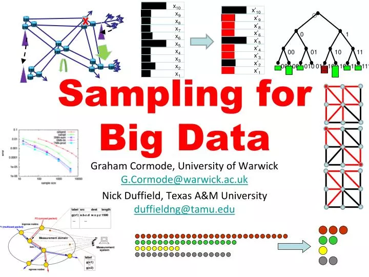
1.  0 1 00 01 10 11 x10 000 001 010 011 100 101 110 111 Sampling for Big Data x9 x8 x7 x6 x5 x4 x3 Graham Cormode, University of WarwickG.Cormode@warwick.ac.uk Nick Duffield, Texas A&M Universityduffieldng@tamu.edu x2 x1 x’10 x’9 x’8 x’6 x’5 x’4 x’3 x’2 x’1

2. Big Data • “Big” data arises in many forms: • Physical Measurements: from science (physics, astronomy) • Medical data: genetic sequences, detailed time series • Activity data: GPS location, social network activity • Business data: customer behavior tracking at fine detail • Common themes: • Data is large, and growing • There are important patterns and trends in the data • We don’t fully know where to lookor how to find them

3. Why Reduce? • Although “big” data is about more than just the volume……most big data is big! • It is not always possible to store the data in full • Many applications (telecoms, ISPs, search engines) can’t keep everything • It is inconvenient to work with data in full • Just because we can, doesn’t mean we should • It is faster to work with a compact summary • Better to explore data on a laptop than a cluster

4. Why Sample? • Sampling has an intuitive semantics • We obtain a smaller data set with the same structure • Estimating on a sample is often straightforward • Run the analysis on the sample that you would on the full data • Some rescaling/reweighting may be necessary • Sampling is general and agnostic to the analysis to be done • Other summary methods only work for certain computations • Though sampling can be tuned to optimize some criteria • Sampling is (usually) easy to understand • So prevalent that we have an intuition about sampling

5. Alternatives to Sampling • Sampling is not the only game in town • Many other data reduction techniques by many names • Dimensionality reduction methods • PCA, SVD, eigenvalue/eigenvector decompositions • Costly and slow to perform on big data • “Sketching” techniques for streams of data • Hash based summaries via random projections • Complex to understand and limited in function • Other transform/dictionary based summarization methods • Wavelets, Fourier Transform, DCT, Histograms • Not incrementally updatable, high overhead • All worthy of study – in other tutorials

6. Health Warning: contains probabilities • Will avoid detailed probability calculations, aim to give high level descriptions and intuition • But some probability basics are assumed • Concepts of probability, expectation, variance of random variables • Allude to concentration of measure (Exponential/Chernoff bounds) • Feel free to ask questions about technical details along the way

7. Outline • Motivating application: sampling in large ISP networks • Basics of sampling: concepts and estimation • Stream sampling: uniform and weighted case • Variations: Concise sampling, sample and hold, sketch guided BREAK • Advanced stream sampling: sampling as cost optimization • VarOpt, priority, structure aware, and stable sampling • Hashing and coordination • Bottom-k, consistent sampling and sketch-based sampling • Graph sampling • Node, edge and subgraph sampling • Conclusion and future directions

8. Sampling as a Mediator of Constraints Data Characteristics (Heavy Tails, Correlations) Sampling Resource Constraints (Bandwidth, Storage, CPU) Query Requirements (Ad Hoc, Accuracy, Aggregates, Speed)

9. Motivating Application: ISP Data • Will motivate many results with application to ISPs • Many reasons to use such examples: • Expertise: tutors from telecoms world • Demand: many sampling methods developed in response to ISP needs • Practice: sampling widely used in ISP monitoring, built into routers • Prescience: ISPs were first to hit many “big data” problems • Variety: many different places where sampling is needed • First, a crash-course on ISP networks…

10. Structure of Large ISP Networks Peering with other ISPs City-levelRouter Centers Access Networks: Wireless, DSL, IPTV Backbone Links Downstream ISP and business customers Network Management & Administration Service and Datacenters

11. Measuring the ISP Network: Data Sources • Protocol Monitoring: • Routers, Wireless • Status Reports: • Device failures and transitions Peering Router Centers Access Backbone • Loss & Latency Roundtrip to edge Loss& Latency Active probing Link Traffic Rates Aggregated per router interface Business Traffic Matrices Flow records from routers • Customer Care Logs • Reactive indicators of network performance Management Datacenters

12. Why Summarize (ISP) Big Data? • When transmission bandwidth for measurements is limited • Not such a big issue in ISPs with in-band collection • Typically raw accumulation is not feasible (even for nation states) • High rate streaming data • Maintain historical summaries for baselining, time series analysis • To facilitate fast queries • When infeasible to run exploratory queries over full data • As part of hierarchical query infrastructure: • Maintain full data over limited duration window • Drill down into full data through one or more layers of summarization Sampling has been proved to be a flexible method to accomplish this

13. Data Scale:Summarization and Sampling

14. Traffic Measurement in the ISP Network Router Centers Access Backbone Business Traffic Matrices Flow records from routers Management Datacenters

15. time flow 4 flow 1 flow 2 flow 3 Massive Dataset: Flow Records • IP Flow: set of packets with common key observed close in time • Flow Key: IP src/dst address, TCP/UDP ports, ToS,… [64 to 104+ bits] • Flow Records: • Protocol level summaries of flows, compiled and exported by routers • Flow key, packet and byte counts, first/last packet time, some router state • Realizations: Cisco Netflow, IETF Standards • Scale: 100’s TeraBytesof flow records daily are generated in a large ISP • Used to manage network over range of timescales: • Capacity planning (months),…., detecting network attacks (seconds) • Analysis tasks • Easy: timeseries of predetermined aggregates (e.g. address prefixes) • Hard: fast queries over exploratory selectors, history, communications subgraphs

16. Flows, Flow Records and Sampling • Two types of sampling used in practice for internet traffic: • Sampling packet stream in router prior to forming flow records • Limits the rate of lookups of packet key in flow cache • Realized as Packet Sampled NetFlow (more later…) • Downstream sampling of flow records in collection infrastructure • Limits transmission bandwidth, storage requirements • Realized in ISP measurement collection infrastructure (more later…) • Two cases illustrative of general property • Different underlying distributions require different sample designs • Statistical optimality sometimes limited by implementation constraints • Availability of router storage, processing cycles

17. Abstraction: Keyed Data Streams • Data Model: objects are keyed weights • Objects (x,k): Weightx; key k • Example 1: objects = packets, x = bytes, k = key (source/destination) • Example 2: objects = flows, x = packets or bytes, k = key • Example 3: objects = account updates, x = credit/debit, k = account ID • Stream of keyed weights, {(xi ,ki): i = 1,2,…,n} • Generic query: subset sums • X(S) = ΣiSxifor S  {1,2,…,n} i.e. total weight of index subset S • Typically S = S(K) = {i: ki K} : objects with keys in K • Example 1, 2: X(S(K)) = total bytes to given IP dest address / UDP port • Example 3: X(S(K)) = total balance change over set of accounts • Aim: Compute fixed size summary of stream that can be used to estimate arbitrary subset sums with known error bounds

18. Inclusion Sampling and Estimation • Horvitz-Thompson Estimation: • Object of size xi sampled with probability pi • Unbiased estimate x’i= xi / pi(if sampled), 0 if not sampled: E[x’i] = xi • Linearity: • Estimate of subset sum = sum of matching estimates • Subset sum X(S)= iSxiis estimated byX’(S) = iSx’i • Accuracy: • Exponential Bounds: Pr[ |X’(S) - X(S)| > δX(S)] ≤ exp[-g(δ)X(S)] • Confidence intervals: X(S) [X-() , X+()] with probability 1 -  • Futureproof: • Don’t need to know queries at time of sampling • “Where/where did that suspicious UDP port first become so active?” • “Which is the most active IP address within than anomalous subnet?” • Retrospective estimate: subset sum over relevant keyset

19. Independent Stream Sampling • Bernoulli Sampling • IID sampling of objects with some probability p • Sampled weight x has HT estimate x/p • Poisson Sampling • Weight xi sampled with probability pi ; HT estimate xi / pi • When to use Poisson vs. Bernoulli sampling? • Elephants and mice: Poisson allows probability to depend on weight… • What is best choice of probabilities for given stream {xi} ?

20. Bernoulli Sampling • The easiest possible case of sampling: all weights are 1 • N objects, and want to sample k from them uniformly • Each possible subset of k should be equally likely • Uniformly sample an index from N (without replacement) k times • Some subtleties: truly random numbers from [1…N] on a computer? • Assume that random number generators are good enough • Common trick in DB: assign a random number to each item and sort • Costly if N is very big, but so is random access • Interesting problem: take a single linear scan of data to draw sample • Streaming model of computation: see each element once • Application: IP flow sampling, too many (for us) to store • (For a while) common tech interview question

21. Reservoir Sampling “Reservoir sampling” described by [Knuth 69, 81]; enhancements [Vitter 85] • Fixed size k uniform sample from arbitrary size N stream in one pass • No need to know stream size in advance • Include first k items w.p. 1 • Include item n > k with probability pn = k/n, n > k • Pick j uniformly from {1,2,…,n} • If j ≤ k, swap item n into location j in reservoir, discard replaced item • Neat proof shows the uniformity of the sampling method: • Let Sn = sample set after n arrivals m (< n) New item: selection probability Prob[n Sn] = pn := k/n n k=7 Previously sampled item: induction m Sn-1w.p. pn-1 m Snw.p. pn-1 * (1 – pn / k) = pn

22. Reservoir Sampling: Skip Counting • Simple approach: check each item in turn • O(1) per item: • Fine if computation time < interarrival time • Otherwise build up computation backlog O(N) • Better: “skip counting” • Find random index m(n) of next selection > n • Distribution: Prob[m(n) ≤ m] = 1 - (1-pn+1)*(1-pn+2)*…*(1-pm) • Expected number of selections from stream is k + Σk<m≤N pm= k + Σk<m≤Nk/m = O(k ( 1 + ln (N/k) )) • Vitter’85 provided algorithm with this average running time

23. Reservoir Sampling via Order Sampling • Order sampling a.k.a. bottom-k sample, min-hashing • Uniform sampling of stream into reservoir of size k • Each arrival n: generate one-time random value rn U[0,1] • rnalso known as hash, rank, tag… • Store k items with the smallest random tags 0.391 0.908 0.291 0.555 0.619 0.273 • Each item has same chance of least tag, so uniform • Fast to implement via priority queue • Can run on multiple input streams separately, then merge

24. Handling Weights • So far: uniform sampling from a stream using a reservoir • Extend to non-uniform sampling from weighted streams • Easy case: k=1 • Sampling probability p(n) = xn/Wn where Wn = Si=1n xi • k>1 is harder • Can have elements with large weight: would be sampled with prob 1? • Number of different weighted order-sampling schemes proposed to realize desired distributional objectives • Rank rn= f(un, xn ) for some function f and un U[0,1] • k-mins sketches [Cohen 1997], Bottom-k sketches [Cohen Kaplan 2007] • [Rosen 1972], Weighted random sampling [EfraimidisSpirakis2006] • Order PPS Sampling [Ohlsson 1990, Rosen 1997] • Priority Sampling [Duffield Lund Thorup 2004], [Alon+DLT 2005]

25. Weighted random sampling • Weighted random sampling [EfraimidisSpirakis 06]generalizes min-wise • For each item draw rnuniformly at random in range [0,1] • Compute the ‘tag’ of an item as rn(1/xn) • Keep the items with the k smallest tags • Can prove the correctness of the exponential sampling distribution • Can also make efficient via skip counting ideas

26. Priority Sampling • Each item xi given priority zi = xi / riwith rnuniform random in (0,1] • Maintain reservoir of k+1 items (xi , zi ) of highest priority • Estimation • Let z* = (k+1)st highest priority • Top-k priority items: weight estimate x’I = max{ xi , z* } • All other items: weight estimate zero • Statistics and bounds • x’Iunbiased; zero covariance: Cov[x’i , x’j ] = 0 for i≠j • Relative variance for any subset sum ≤ 1/(k-1) [Szegedy, 2006]

27. Priority Sampling in Databases • One Time Sample Preparation • Compute priorities of all items, sort in decreasing priority order • No discard • Sample and Estimate • Estimate any subset sum X(S) =iSxiby X’(S) = iSx’I for some S’ S • Method: select items in decreasing priority order • Two variants: bounded variance or complexity • S’ = first k items from S: relative variance bounded ≤ 1/(k-1) • x’I= max{ xi, z* } where z* = (k+1)st highest priority in S • S’ = items from S in first k: execution time O(k) • x’I= max{ xi , z* } where z* = (k+1)st highest priority [Alon et. al., 2005]

28. Making Stream Samples Smarter • Observation: we see the whole stream, even if we can’t store it • Can keep more information about sampled items if repeated • Simple information: if item sampled, count all repeats • Counting Samples [Gibbons & Mattias 98] • Sample new items with fixed probability p, count repeats as ci • Unbiased estimate of total count: 1/p + (ci – 1) • Sample and Hold [Estan & Varghese 02]: generalize to weighted keys • New key with weight bsampled with probability 1 - (1-p)b • Lower variance compared with independent sampling • But sample size will grow as pn • Adaptive sample and hold: reduce p when needed • “Sticky sampling”: geometric decreases in p[Manku, Motwani 02] • Much subsequent work tuning decrease in p to maintain sample size

29. Sketch Guided Sampling • Go further: avoid sampling the heavy keys as much • Uniform sampling will pick from the heavy keys again and again • Idea: use an oracle to tell when a key is heavy [Kumar Xu 06] • Adjust sampling probability accordingly • Can use a “sketch” data structure to play the role of oracle • Like a hash table with collisions, tracks approximate frequencies • E.g. (Counting) Bloom Filters, Count-Min Sketch • Track probability with which key is sampled, use HT estimators • Set probability of sampling key with (estimated) weight w as 1/(1 + ew) for parameter e : decreases as w increases • Decreasing e improves accuracy, increases sample size

30. Challenges for Smart Stream Sampling • Current router constraints • Flow tables maintained in fast expensive SRAM • To support per packet key lookup at line rate • Implementation requirements • Sample and Hold: still need per packet lookup • Sampled NetFlow: (uniform) sampling reduces lookup rate • Easier to implement despite inferior statistical properties • Long development times to realize new sampling algorithms • Similar concerns affect sampling in other applications • Processing large amounts of data needs awareness of hardware • Uniform sampling means no coordination needed in distributed setting

31. Future for Smarter Stream Sampling • Software Defined Networking • Current: proprietary software running on special vendor equipment • Future: open software and protocols on commodity hardware • Potentially offers flexibility in traffic measurement • Allocate system resources to measurement tasks as needed • Dynamic reconfiguration, fine grained tuning of sampling • Stateful packet inspection and sampling for network security • Technical challenges: • High rate packet processing in software • Transparent support from commodity hardware • OpenSketch: [Yu, Jose, Miao, 2013] • Same issues in other applications: use of commodity programmable HW

32. Stream Sampling:Sampling as Cost Optimization

33. Matching Data to Sampling Analysis • Generic problem 1: Counting objects: weight xi = 1 Bernoulli (uniform) sampling with probability p works fine • Estimated subset count X’(S) = #{samples in S} / p • Relative Variance (X’(S)) = (1/p -1)/X(S) • given p, get any desired accuracy for large enough S • Generic problem 2: xi in Pareto distribution, a.k.a. 80-20 law • Small proportion of objects possess a large proportion of total weight • How to best to sample objects to accurately estimate weight? • Uniform sampling? • likely to omit heavy objects  big hit on accuracy • making selection set S large doesn’t help • Select m largest objects ? • biased & smaller objects systematically ignored

34. Heavy Tails in the Internet and Beyond • Files sizes in storage • Bytes and packets per network flow • Degree distributions in web graph, social networks

35. Non-Uniform Sampling • Extensive literature: see book by [Tille, “Sampling Algorithms”, 2006] • Predates “Big Data” • Focus on statistical properties, not so much computational • IPPS: Inclusion Probability Proportional to Size • Variance Optimal for HT Estimation • Sampling probabilities for multivariate version: [Chao 1982, Tille 1996] • Efficient stream sampling algorithm: [Cohen et. al. 2009]

36. Costs of Non-Uniform Sampling • Independent sampling from n objects with weights {x1,… ,xn} • Goal: find the “best” sampling probabilities {p1, … ,pn} • Horvitz-Thompson: unbiased estimation of each xi by • Two costs to balance: • Estimation Variance: Var(x’i) = x2i (1/pi – 1) • Expected Sample Size: ipi • Minimize Linear Combination Cost: i(xi2(1/pi –1) + z2 pi) • z expresses relative importance of small sample vs. small variance

37. Minimal Cost Sampling: IPPS IPPS: Inclusion Probability Proportional to Size • MinimizeCost i(xi2(1/pi – 1) + z2 pi) subject to 1 ≥ pi≥ 0 • Solution: pi = pz(xi) = min{1, xi /z} • small objects (xi < z) selected with probability proportional to size • large objects (xi≥ z) selected with probability 1 • Call z the “sampling threshold” • Unbiased estimator xi/pi =max{xi , z} • Perhaps reminiscent of importancesampling, but not the same: • make no assumptions concerningdistribution of the x pz(x) 1 x z

38. Error Estimates and Bounds • Variance Based: • HT sampling variance for single object of weight xi • Var(x’i) = x2i (1/pi– 1) = x2i (1/min{1,xi/z} – 1) ≤ z xi • Subset sum X(S)= iSxiis estimated byX’(S) = iSx’i • Var(X’(S)) ≤ z X(S) • Exponential Bounds • E.g. Prob[X’(S) = 0] ≤ exp(-X(S) / z ) • Bounds are simple and powerful • depend only on subset sum X(S), not individual constituents

39. Sampled IP Traffic Measurements • Packet Sampled NetFlow • Sample packet stream in router to limit rate of key lookup: uniform 1/N • Aggregate sampled packets into flow records by key • Model: packet stream of (key, bytesize) pairs { (bi, ki) } • Packet sampled flow record (b,k) where b = Σ {bi : i sampled ∧ki = k} • HT estimate b*N of total bytes in flow • Downstream sampling of flow records in measurement infrastructure • IPPS sampling, probability min{1, b*N/z} • Chained variance bound for any subset sum X of flows • Var(X’) ≤ (z + Nbmax) X where bmax= maximum packet byte size • Regardless of how packets are distributed amongst flows [Duffield, Lund, Thorup, IEEE ToIT, 2004]

40. Estimation Accuracy in Practice • Estimate any subset sum comprising at least some fraction f of weight • Suppose: sample size m • Analysis: typical estimation error ε (relative standard deviation) obeys • 2**16 = storage needed for aggregates over 16 bit address prefixes • But sampling gives more flexibility to estimate traffic within aggregates m Estimate fraction f = 0.1% with typical relative error 12%:

41. Heavy Hitters: Exact vs. Aggregate vs. Sampled • Sampling does not tell you where the interesting features are • But does speed up the ability to find them with existing tools • Example: Heavy Hitter Detection • Setting: Flow records reporting 10GB/s traffic stream • Aim: find Heavy Hitters = IP prefixes comprising ≥ 0.1% of traffic • Response time needed: 5 minute • Compare: • Exact: 10GB/s x 5 minutes yields upwards of 300M flow records • 64k aggregates over 16 bit prefixes: no deeper drill-down possible • Sampled: 64k flow records: any aggregate ≥ 0.1% accurate to 10% Exact Aggregate Sampled

42. Cost Optimization for Sampling Several different approaches optimize for different objectives: • Fixed Sample Size IPPS Sample • Variance Optimal sampling: minimal variance unbiased estimation • Structure Aware Sampling • Improve estimation accuracy for subnet queries using topological cost • Fair Sampling • Adaptively balance sampling budget over subpopulations of flows • Uniform estimation accuracy regardless of subpopulation size • Stable Sampling • Increase stability of sample set by imposing cost on changes

43. IPPS Stream Reservoir Sampling • Each arriving item: • Provisionally include item in reservoir • If m+1 items, discard 1 item randomly • Calculate threshold z to sample mitems on average: zsolves ipz(xi) = m • Discard item i with probability qi =1 – pz(xi) • Adjust m surviving xiwith Horvitz-Thompson x’i = xi / pi = max{xi,z} • Efficient Implementation: • Computational cost O(log m ) per item, amortized cost O(log log m) [Cohen, Duffield, Lund, Kaplan, Thorup; SODA 2009, SIAM J. Comput. 2011] x10 1 x9 Recalculatethreshold z: Recalculate Discard probs: x8 Adjust weights: x7 x6 x5 z x4 x3 x2 0 x1 x10 x’10 x’9 x9 x’8 x8 Example: m=9 x7 x6 x’6 x’5 x5 x4 x’4 x3 x’3 x2 x’2 x1 x’1

44. Structure (Un)Aware Sampling • Sampling is oblivious to structure in keys (IP address hierarchy) • Estimation disperses the weight of discarded items to surviving samples • Queries structure aware: subset sums over related keys (IP subnets) • Accuracy on LHS is decreased by discarding weight on RHS  0 1 00 01 10 11 000 001 010 011 100 101 110 111

45. Localizing Weight Redistribution • Initial weight set {xi : iS} for some S  Ω • E.g.Ω= possible IP addresses, S =observed IP addresses • Attribute “range cost” C({xi : iR}) for each weight subset RS • Possible factors for Range Cost: • Sampling variance • Topology e.g. height of lowest common ancestor • Heuristics: R* = Nearest Neighbor {xi , xj} of minimal xixj • Sample k items from S: • Progressively remove one item from subset with minimal range cost: • While(|S| > k) • Find R*S of minimal range cost. • Remove a weight from R* w/ VarOpt [Cohen, Cormode, Duffield; PVLDB 2011] No change outside subtree belowclosest ancestor  0 1 00 01 10 11 Order of magnitude reduction in average subnet error vs. VarOpt 000 001 010 011 100 101 110 111

46. Fair Sampling Across Subpopulations • Analysis queries often focus on specific subpopulations • E.g. networking: different customers, user applications, network paths • Wide variation in subpopulation size • 5 orders of magnitude variation in traffic on interfaces of access router • If uniform sampling across subpopulations: • Poor estimation accuracy on subset sums within small subpopulations Sample Color = subpopulation , = interesting items • occurrence proportional to subpopulation size Uniform Sampling across subpopulations: • Difficult to track proportion of interesting items within small subpopulations:

47. Fair Sampling Across Subpopulations • Minimize relative variance by sharing budget m over subpopulations • Total nobjectsin subpopulations n1,…,nd with ini=n • Allocate budget mi to each subpopulation ni with imi=m • Minimize average population relative variance R = const. i1/mi • Theorem: • R minimized when {mi} are Max-Min Fair share of m under demands {ni} • Streaming • Problem: don’t know subpopulation sizes {ni} in advance • Solution: progressive fair sharing as reservoir sample • Provisionally include each arrival • Discard 1 item as VarOptsample from any maximal subpopulation • Theorem [Duffield; Sigmetrics 2012]: • Max-Min Fair at all times; equality in distribution with VarOpt samples {mifrom ni}

48. Stable Sampling • Setting: Sampling a population over successive periods • Sample independently at each time period? • Cost associated with sample churn • Time series analysis of set of relatively stable keys • Find sampling probabilities through cost minimization • Minimize Cost = Estimation Variance + z * E[#Churn] • Size m sample with maximal expected churn D • weights {xi}, previous sampling probabilities {pi} • find new sampling probabilities {qi} to minimize cost of taking m samples • Minimize ix2i / qisubject to 1 ≥ qi≥ 0, I qi = m and I | pi– qi | ≤D [Cohen, Cormode, Duffield, Lund 13]

49. Summary of Part 1 • Sampling as a powerful, general summarization technique • Unbiased estimation via Horvitz-Thompson estimators • Sampling from streams of data • Uniform sampling: reservoir sampling • Weighted generalizations: sample and hold, counting samples • Advances in stream sampling • The cost principle for sample design, and IPPS methods • Threshold, priority and VarOpt sampling • Extending the cost principle: • structure aware, fair sampling, stable sampling, sketch guided

50. Outline • Motivating application: sampling in large ISP networks • Basics of sampling: concepts and estimation • Stream sampling: uniform and weighted case • Variations: Concise sampling, sample and hold, sketch guided BREAK • Advanced stream sampling: sampling as cost optimization • VarOpt, priority, structure aware, and stable sampling • Hashing and coordination • Bottom-k, consistent sampling and sketch-based sampling • Graph sampling • Node, edge and subgraph sampling • Conclusion and future directions