Download
1 / 26
260 likes | 381 Views
CS473-Algorithms I. Lecture 14-A Graph Searching: Breadth-First Search. Graph Searching: Breadth-First Search Graph G ( V , E ), directed or undirected with adjacency list repres. GOAL: Systematically explores edges of G to discover every vertex reachable from the source vertex s

E N D
CS473-Algorithms I Lecture 14-A Graph Searching: Breadth-First Search Lecture 14
Graph Searching: Breadth-First Search • Graph G(V, E), directed or undirected with adjacency list repres. • GOAL: Systematically explores edges of G to • discover every vertex reachable from the source vertex s • compute the shortest path distance of every vertex from the source vertex s • produce a breadth-first tree (BFT)G with root s • BFT contains all vertices reachable from s • the unique path from any vertex v to s in G constitutes a shortest path from s to v in G • IDEA: Expanding frontier across the breadth -greedy- • propagate a wave 1 edge-distance at a time • using a FIFO queue: O(1) time to update pointers to both ends Lecture 14
Breadth-First Search Algorithm • Maintains the following fields for each u V • color[u]: color of u • WHITE : not discovered yet • GRAY : discovered and to be or being processed • BLACK: discovered and processed • [u]: parent of u (NIL of u s or u is not discovered yet) • d[u]: distance of u from s • Processing a vertex scanning its adjacency list Lecture 14
Breadth-First Search Algorithm • BFS(G, s) • for each u V {s} do • color[u] WHITE • [u] NIL; d [u] • color[s] GRAY • [s] NIL; d [s] 0 • Q {s} • while Q do • u head[Q] • for each v in Adj[u] do • if color[v] WHITE then • color[v] GRAY • [v] u • d [v] d [u] 1 • ENQUEUE(Q, v) • DEQUEUE(Q) • color[u] BLACK Lecture 14
Breadth-First Search Sample Graph: FIFO just after queue Qprocessing vertex a - Lecture 14
Breadth-First Search FIFO just after queue Qprocessing vertex a - a,b,c a Lecture 14
Breadth-First Search FIFO just after queue Qprocessing vertex a - a,b,c a a,b,c,f b Lecture 14
Breadth-First Search FIFO just after queue Qprocessing vertex a - a,b,c a a,b,c,f b a,b,c,f,e c Lecture 14
Breadth-First Search FIFO just after queue Qprocessing vertex a - a,b,c a a,b,c,f b a,b,c,f,e c a,b,c,f,e,g,h f Lecture 14
Breadth-First Search FIFO just after queue Qprocessing vertex a - a,b,c a a,b,c,f b a,b,c,f,e c a,b,c,f,e,g,h f a,b,c,f,e,g,h,d,i e all distances are filled in after processing e Lecture 14
Breadth-First Search FIFO just after queue Qprocessing vertex a - a,b,c a a,b,c,f b a,b,c,f,e c a,b,c,f,e,g,h f a,b,c,f,e,g,h,d,i g Lecture 14
Breadth-First Search FIFO just after queue Qprocessing vertex a - a,b,c a a,b,c,f b a,b,c,f,e c a,b,c,f,e,g,h f a,b,c,f,e,g,h,d,i h Lecture 14
Breadth-First Search FIFO just after queue Qprocessing vertex a - a,b,c a a,b,c,f b a,b,c,f,e c a,b,c,f,e,g,h f a,b,c,f,e,g,h,d,i d Lecture 14
Breadth-First Search FIFO just after queue Qprocessing vertex a - a,b,c a a,b,c,f b a,b,c,f,e c a,b,c,f,e,g,h f a,b,c,f,e,g,h,d,i i algorithm terminates: all vertices are processed Lecture 14
Breadth-First Search Algorithm • Running time: O(VE) considered linear time in graphs • initialization: (V) • queue operations: O(V) • each vertex enqueued and dequeued at most once • both enqueue and dequeue operations take O(1) time • processing gray vertices: O(E) • each vertex is processed at most once and Lecture 14
Theorems Related to BFS • DEF: (s, v) shortest path distance from s to v • LEMMA 1: for any s V & (u, v) E; (s, v) (s, u) 1 • For any BFS(G,s) run on G(V,E) • LEMMA 2:d [v] (s, v) v V • LEMMA 3: at any time of BFS, the queue Qv1, v2, …, vr satisfies • d [vr] d [v1] 1 • d [vi] d [vi1], for i1, 2, …, r 1 • THM1:BFS(G, s) achieves the following • discovers every v V where s v (i.e., v is reachable from s) • upon termination, d [v] (s, v) v V • for any v s & s v; sp(s,[v]) ([v], v) is a sp(s, v) Lecture 14
Proofs of BFS Theorems • DEF: shortest path distance (s, v) from s to v • (s, v) minimum number of edges in any path from s to v • if no such path exists (i.e., v is not reachable from s) • L1: for any s V & (u, v) E; (s, v) (s, u) 1 • PROOF: s u s v. Then, • consider the path p(s, v) sp(s, u) (u, v) • |p(s, v)| | sp(s, u) | 1 (s, u) 1 • therefore, (s, v) |p(s, v)| (s, u) 1 sp(s, u) p(s, v) Lecture 14
Proofs of BFS Theorems • DEF: shortest path distance (s, v) from s to v • (s, v) minimum number of edges in any path from s to v • L1: for any s V & (u, v) E; (s, v) (s, u) 1 • C1 of L1: if G(V,E) is undirected then (u, v) E (v, u) E • (s, v) (s, u) 1 and (s, u) (s, v) 1 • (s, u) 1 (s, v) (s, u) 1 and • (s, v) 1 (s, u) (s, v) 1 • (s, u) & (s, v) differ by at most 1 sp(s, u) sp(s, v) Lecture 14
Proofs of BFS Theorems • L2: upon termination of BFS(G, s) on G(V,E); • d [v] (s, v) v V • PROOF: by induction on the number of ENQUEUE operations • basis: immediately after 1st enqueue operation ENQ(Q, s): d [s] (s, s) • hypothesis:d [v] (s, v) for all v inserted into Q • induction: consider a white vertex v discovered during scanning Adj[u] • d [v] d [u] 1 due to the assignment statement • (s, u) 1 due to the inductive hypothesis since u Q • (s, v) due to L1 • vertex vis then enqueued and it is never enqueued again • d [v] never changes again, maintaining inductive hypothesis Lecture 14
Proofs of BFS Theorems • L3: Let Q v1, v2, …, vr during the execution of BFS(G, s), then, • d [vr] d [v1] 1 and d [vi] d [vi1] for i 1, 2, …, r1 • PROOF: by induction on the number of QUEUE operations • basis: lemma holds when Q {s} • hypothesis: lemma holds for a particular Q (i.e., after a certain # of QUEUE operations) • induction: must prove lemma holds after both DEQUEUE & ENQUEUE operations • DEQUEUE(Q): Q v1, v2, …, vr Q v2, v3, …, vr • d [vr] d [v1] 1 & d [v1] d [v2] in Q d [vr] d [v2] 1 inQ • d [vi] d [vi1] for i 1, 2, …, r1 in Q d [vi] d [vi1] for i 2, …, r1 inQ Lecture 14
Proofs of BFS Theorems • ENQUEUE(Q, v): Q v1, v2, …, vr • Q v1, v2, …, vr , vr1v • v was encountered during scanning Adj[u] where u v1 • thus, d [vr1] d [v] d [u] 1 d [v1] 1 d [vr1] d [v1] 1 inQ • but d [vr] d [v1] 1 d [vr1] • d [vr1] d [v1] 1 and d [vr] d [vr1] in Q C3 of L3 (monotonicity property): if: the vertices are enqueued in the order v1, v2, …, vn then: the sequence of distances is monotonically increasing, i.e., d [v1] d [v2] ………. d [vn] Lecture 14
Proofs of BFS Theorems • THM (correctness of BFS): BFS(G, s) achieves the following on G(V,E) • discovers everyv V wheres v • upon termination:d [v] (s, v) v V • for any v s & s v; sp(s,[v]) ([v], v) sp(s, v) • PROOF: by induction on k, whereVk {v V: (s, v) k} • hypothesis: for each v Vk, exactly one point during execution of BFS at which color[v] GRAY, d [v] k, [v] u Vk1, and then ENQUEUE(Q, v) • basis:for k 0 since V0 {s}; color[s] GRAY, d [s] 0 and ENQUEUE(Q, s) • induction:must prove hypothesis holds for each v Vk1 Lecture 14
Proofs of BFS Theorems • Consider an arbitrary vertex v Vk1, where k 0 • monotonicity (L3) d [v] k 1 (L2) + inductive hypothesis • v must be discovered after all vertices in Vk were enqueued • since (s, v) k 1, u Vk such that (u, v) E • let uVk be the first such vertex grayed (must happen due to hyp.) • u head(Q) will be ultimately executed since BFS enqueues every grayed vertex • v will be discovered during scanning Adj[u] color[v]WHITE since v isn’t adjacent to any vertex in Vj for j<k • color[v] GRAY, d [v] d [u] 1, [v] u • then, ENQUEUE(Q, v) thus proving the inductive hypothesis • To conclude the proof • if v Vk1 then due to above inductive proof [v] Vk • thus sp(s, [v]) ([v], v) is a shortest path from s to v Lecture 14
Theorems Related to BFS • DEF: (s, v) shortest path distance from s to v • LEMMA 1: for any s V & (u, v) E; (s, v) (s, u) 1 • For any BFS(G,s) run on G(V,E) • LEMMA 2:d [v] (s, v) v V • LEMMA 3: at any time of BFS, the queue Qv1, v2, …, vr satisfies • d [vr] d [v1] 1 • d [vi] d [vi1], for i1, 2, …, r 1 • THM1:BFS(G, s) achieves the following • discovers every v V where s v (i.e., v is reachable from s) • upon termination, d [v] (s, v) v V • for any v s & s v; sp(s,[v]) ([v], v) is a sp(s, v) Lecture 14
Breadth-First Tree Generated by BFS • LEMMA 4:predecessor subgraphG(V, E) generated by BFS(G, s) , where V {v V: [v] NIL}{s} and • E {([v],v) E: v V {s}} • is a breadth-first tree such that • V consists of all vertices in V that are reachable from s • v V , unique path p(v, s) in G constitutes a sp(s, v) in G PRINT-PATH(G, s, v) ifv sthen print s else if[v] NIL then print no “sv path” else PRINT-PATH(G, s, [v] ) print v Prints out vertices on a sv shortest path Lecture 14
Breadth-First Tree Generated by BFS BFS(G,a) terminated BFT generated by BFS(G,a) Lecture 14