Download
1 / 9
230 likes | 771 Views
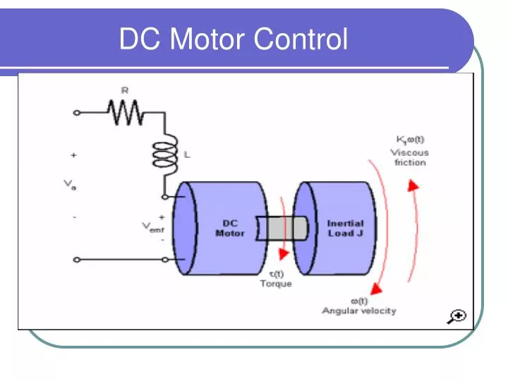
DC Motor Control. Control Figure. Motor Constants. For this example, the physical constants are: R = 2.0; % Ohms L = 0.5; % Henrys Km = 0.1; Kb = 0.1; % torque and back emf constants Kf = 0.2; % Nms J = 0.02; % kg.m^2/s^2. h1 = tf(Km,[L R]); % armature

E N D
Motor Constants For this example, the physical constants are: R = 2.0; % Ohms L = 0.5; % Henrys Km = 0.1; Kb = 0.1; % torque and back emf constants Kf = 0.2; % Nms J = 0.02; % kg.m^2/s^2
h1 = tf(Km,[L R]); % armature h2 = tf(1,[J Kf]); % eqn of motion dcm = ss(h2) * [h1 , 1]; % w = h2 * (h1*Va + Td) dcm = feedback(dcm,Kb,1,1); % close back emf loop step (dcm(1))
Feed forward You can use this simple feedforward control structure to command the angular velocity w to a given value w_ref.
Feed forward Kff = 1/dcgain(dcm(1)) To evaluate the feedforward design in the face of load disturbances, simulate the response to a step command w_ref=1 with a disturbance Td = -0.1Nm between t=5 and t=10 seconds:
t = 0:0.1:15; Td = -0.1 * (t>5 & t<10); % load disturbance u = [ones(size(t)) ; Td]; % w_ref=1 and Td cl_ff = dcm * diag([Kff,1]); % add feedforward gain set(cl_ff,'InputName',{'w_ref','Td'},'OutputName','w'); h = lsimplot(cl_ff,u,t); title('Setpoint tracking and disturbance rejection') legend('cl\_ff') % Annotate plot line([5,5],[.2,.3]); line([10,10],[.2,.3]); text(7.5,.25,{'disturbance','T_d = -0.1Nm'},... 'vertic','middle','horiz','center','color','r');
http://www.mathworks.com/products/control/demos.html?file=/products/demos/shipping/control/dcdemo.htmlhttp://www.mathworks.com/products/control/demos.html?file=/products/demos/shipping/control/dcdemo.html