Download
1 / 17
170 likes | 258 Views
This study conducts a detailed kinematical analysis of solar wind outflows using STEREO/EUVI images, focusing on intensity fluctuations and speed measurements. Data from various telescopes like SOHO/EIT, TRACE, HINODE/EIS, and Hinode XRT are used to validate observations. The research investigates contributions of outflows to the slow solar wind and their association with active regions. Techniques such as wavelet processing and force-free magnetic field modeling are employed to analyze plasma flows guided by magnetic fields in the solar corona. The study aims to enhance our understanding of solar wind formation processes and the dynamics of coronal structures.

E N D
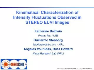
Kinematical Characterization of Intensity Fluctuations Observed in STEREO EUVI Images Katherine Baldwin Praxis, Inc. / NRL Guillermo Stenborg Interferometrics, Inc. / NRL Angelos Vourlidas, Russ Howard Naval Research Lab (NRL)
Motivation - Robbrecht Waves Slow Magnetoacoustic Waves in Coronal Loops: EIT and TRACE E. Robbrecht, E. Verwichte, D. Berghmans, J. Hochedez, S. Poedts, V. Nakariakov A&A, Vol 370, pp. 591-601, 2001. Telescopes: SOHO/EIT and TRACE Projected Speed: 65 - 150 km/s True Speed: ?? • May 13th, 1998 JOP Campaign.
Motivation - Doschek Outflows • Outflows from the Sun somehow make up the slow solar wind. • Doppler-shifted EIS measurements to validate result. • Also, analyzes a Dec 11, 2007 AR. • Top: FeXII 195.12 A intensity for August 23, 2007 AR • Bottom: Doppler Map (blue is towards the observer) obtained with the Extreme-ultraviolet Imaging Spectrometer (EIS) on the Hinode S/C. Flows and Non-thermal Velocities in Solar Active Regions Observed with Hinode/EIS: A Tracer of Active Region Sources of Heliospheric Magnetic Fields? G. Doschek, H. Warren, J. Mariska, K. Muglach, J. Culhane , H. Hara, T. Watanabe ApJ, Vol 686, pp. 1362-1371, 2008. Telescope: HINODE/EIS LOS Speed: 20-50 km/s True Speed: ?
Motivation - Harra Outflows Outflows at the Edges of Active Regions: Contributions to Solar Wind Formation? L. Harra, T. Sakao, C. Mandrini, H. Hara, S. Imada, P. Young, L. Van Driel-Gesztelyi, D. Baker ApJ, Vol 676, pp. L147-L150, 2008. Telescope: Hinode/XRT LOS Speed: 20-50 km/s True Speed: >100 km/s • The outflows are the major contributor to the slow solar wind. • Outflow occurs at EDGES of active regions. • Large scale loops lie over active region and open to interplanetary space. • Doppler shifted EIS measurements were used as comparison.
Motivation - Marsch Outflows • Photospheric convection drives a global “coronal circulation”. • Most blue shifted occurrences are associated with open or large looped field lines. • Agrees with Harra et al. - mass outflow is contributing to the slow solar wind through “open” field lines. • Using force-free magnetic field model to define open/closed lines. • Loops of specified height (~100,000km) are considered open field lines. Plasma Flows Guided by Strong Magnetic Fields in the Solar Corona E. Marsch, H. Tian, J. Sun, W. Curdt, T. Wiegelmann ApJ, Vol 685, pp. 1262-1269, 2008. Telescope : Hinode/EIS Contours : Force-free magnetic field model LOS Speed: ?? True Speed: ??
Why STEREO/EUVI ? STEREO Advantage • Continuous coverage: • EUVI data does not suffer from small FOV/telemetry problems of Hinode payload. • Suitable temporal resolution • Constantbandpassallows us to follow brightness fluctuations directly, without using Doppler analysis. • 3Dcapabilities • allow true speed calculations.
Does STEREO/EUVI see something similar? March 25, 2008 EUVI 171 B Running difference of wavelet-cleaned images Cadence: 1.5 min Details of the wavelet-cleaning and -enhancing algorithm at A Fresh View of the Extreme-Ultraviolet Corona from the Application of a New Image-Processing Technique Stenborg, G.; Vourlidas, A.; Howard, R. ApJ, Vol 674, Issue 2, pp. 1201-1206. A few words on the wavelet technique
What does STEREO/EUVI observe on February 20, 2007 Outflows at the Edges of Active Regions: Contributions to Solar Wind Formation? L. Harra, T. Sakao, C. Mandrini, H. Hara, S. Imada, P. Young, L. Van Driel-Gesztelyi, D. Baker ApJ, Vol 676, pp. L147-L150, 2008. EUVI B 195 wavelet processed snapshot movie ( time span 8 hs, cadence 10 min ) of a comparable area to that observed by HINODE/XRT HINODE/XRT
August 23, 2007 EUVI B 195 ( 06:55 UT ) wavelet processed snapshot of the disk region shown in Doschek et al paper Full-Disk EUVI B 195 ( 06:55 UT ) wavelet processed intensity image Top: FeXII195.12 A intensity Bottom: Doppler Map (blue is towards the observer) obtained with Hinode/EIS. From Doschek, et al., ApJ, 686, 1362, 2008
December 11, 2007 Also from Doschek, et al., ApJ, 686, 1362, 2008 EUVI B 195: December 11, 2007 AR (03:35 UT) Top: FeXII195.12 A intensity Bottom: Doppler Map (blue is towards the observer) obtained with the HINODE/EIS.
2007/08/23 EUVI B 171 2007/02/20 EUVI B 171 2007/12/09 EUVI B 171 2008/03/25 EUVI B 171 How can we measure the speed of the disturbances? Original idea: Use of Height-Time Maps (J-maps) Sheeley et al. 1999, 2000 available in solar software
K maps • Wavelet-processed images are de-rotated by 8 hour segments. • Paths manually defined by point-and-click on the Region of Interest • K-maps created through each 8 hour segments. Time S/C A Distance along the path S/C A Distance along the path Time • Using the K-maps we are able to find the projected speed of the density enhancements. • Before speed assessment we determine if tracked features remain constant throughout the 8 hour de-rotation period. If not constant, then speed cannot reliably be found.
December 9, 2007 [00:00 UT - 08:00 UT] 95 km/s 120 km/s 115 km/s 100 km/s 95 km/s --- Projected Speed of a sample of intensity variations as they move along the selected ray ---- Kinematical characterization • * On the intensity variations observed along pseudo-open field lines nearby AR A qualitative analysis of the days processed so far showed that, the traveling disturbances are stronger (i.e., better discerned against the background) when: i) closed field lines are nearby apparently open field lines, ii) closed field lines are nearby another closed field lines that end up on different foot points. Example of quantitative analysis The seven cases analyzed (including “on-disk” and “off-limb” cases) result in projected speeds in the range 50 - 140 km/s
Future Work: II) Magnetic Topology • Do these intensity variations exist anywhere else on the disk with closed field lines? • Do the variation exist along plumes with open field lines? • How does magnetic topology relate to flow strengths? • Infer the topology of the magnetic field where the flows are observed by comparing with magnetic field models
Reliability of feature tracking using point-and-click method Accuracy of feature tracking between STEREO-A to STEREO-B Are the flows inside closed (but long) loops or inside open magnetic field extending into the heliosphere? Physical Interpretation: Are the observed intensity fluctuations mass outflows or waves? How is the magnetic field topology where the intensity fluctuations exist? Are the observed intensity fluctuations observed above the polar coronal holes caused by the same mechanism as those observed in pseudo-open field lines nearby AR? Issues to Consider
The 2D “a trous” algorithm 2D B3-spline Wavelet scales 1 to 4 (Wi) Smoothed image corresponding to decomposition based on 25 scales For comparison, smoothed image corresponding to decomposition based on 50 scales Back