Download
1 / 32
320 likes | 627 Views
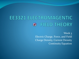
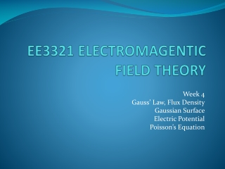
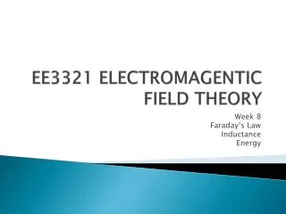
EE3321 ELECTROMAGENTIC FIELD THEORY. Week 6 Magnetic Fields Inverse Square Law Gauss’ Law Biot-Savart’s Law. Magnetic Fields. A magnetic field is a vector field that exerts a magnetic force on moving electric charges and magnetic dipoles (such as permanent magnets).

E N D
EE3321 ELECTROMAGENTIC FIELD THEORY Week 6 Magnetic Fields Inverse Square Law Gauss’ Law Biot-Savart’s Law
Magnetic Fields • A magnetic field is a vector field that exerts a magnetic force on • moving electric charges and • magnetic dipoles (such as permanent magnets). • When placed in a magnetic field, magnetic dipoles tend to align their axes to be parallel with the magnetic field iron filings in the presence of a magnet
Poles • The direction of the magnetic field near the poles of a magnet is revealed by placing compasses nearby. • The magnetic field points towards a magnet's south pole and away from its north pole.
Attraction and Repulsion • Like poles repel each other • Opposite poles attract each other
Earth’s Magnetic Field • First measured by Gauss • The locations are not static • Poles wander as much as 15 km every year
Interplanetary Magnetic Field • There is a magnetic field in deep space
2012 • Earth’s magnetic field deflects most of the radiation from solar flares • Solar flares have a period of 11 years
True North • The magnetic south pole is about 11o from true north
Inverse Square Law • The force between two magnetic poles is given by: where • qm1 and qm2 are the magnitudes of magnetic poles (A m) • μ is the permeability of the intervening medium (N / A2) • r is the separation (m)
Exercise • Suppose that two bar magnets of equal length L are placed end-to-end along the x axis. L x • Show that F = μ (qm)2 / (4 π) –1 [ x –2 + (x + 2L) –2 – 2(x +L) –2 ]
Equivalence • In theory, a magnet can be viewed as a ferromagnetic body with “bound” surface currents that generate the magnetic field much like a solenoid does.
Field Intensity and Flux Density • Magnetic fields are created by • magnetic dipoles, • electric currents, and • changing electric fields. • The magnetic field is characterized by the B and H vectors. Both are related by the permeability (or magnetic constant) μ of the medium
Units • The vector field H is known as the magnetic field intensity or magnetic field strength: • H is measured in Amperes per meter (A/m). • The vector field B is known as magnetic flux density or magnetic induction or simply magnetic field: • B has the units of Teslas (T), equivalent to Webers per square meter (Wb/m²) or volt-seconds per square meter (V s/m²).
Magnetic Mopoles • Magnetic sources are inherently dipole sources • So far we know, one cannot isolate north or south "monopoles“
Broken Duality • An electric charge e in motion generates a magnetic field B • A monopole g in motion would generate an electric field E
Gauss’ Law for Magnetism • Magnetic field lines always form continuous closed loops. The differential form for Gauss' law for magnetism is the following:
Gauss’ Law for Magnetism • The integral form of Gauss' law for magnetism states that where • S is any closed surface (a "closed surface" is the boundary of some three-dimensional volume) • dA is a vector, whose magnitude is the area of an infinitesimal piece of the surface S, and whose direction is the outward-pointing surface normal.
Exercise • The solar wind exerts pressure on the magnetic field of the Earth. • As a result the field is compressed on the side toward the sun and is dragged into space on the side away from the sun. • On the extended side, the magnetic field lines extend beyond 100 Earth radii. • What is the divergence of the field on either side of the Earth?
Gauss’ Law for Magnetism • The left-hand side of this equation is called the net flux of the magnetic field Φ out of the surface, and Gauss' law for magnetism states that it is always zero. • The integral and differential forms of Gauss' law for magnetism are mathematically equivalent, due to the divergence theorem.
Exercise • The magnetic field intensity generated by a small current loop of radius a located at the center of the x-y plane is given by H = Ia2 (aR 2 cosθ + aθ sin θ) / 4R3 • Show that net flux coming out of a Gaussian spherical surface is zero.
Magnetostatics • Magnetostatics is the study of static magnetic fields produced by direct currents. • If all the currents in a system are known, then the magnetic field can be determined from the currents by the Biot-Savart equation. • The Biot–Savart law is used to compute the magnetic field generated by a steady current, for example through a wire, which is constant in time and in which charge is neither building up nor depleting at any point.
Biot-Savart’s Law • The corresponding integral form is where • I is the current • dl is the differential element of the wire in the direction of conventional current • r is the distance between the element and the observation point P
Procedure • The application of this law implicitly relies on the superposition principle for magnetic fields: • the magnetic field is a vector sum of the field created by each infinitesimal section I dl of the wire individually. • Choose a point P in space at which you want to compute the magnetic field. • Holding that point fixed, integrate over the path of the current to find the total magnetic field at that point.
Wire Carrying a Steady Current • In 1820 Biot and Savart announced that the magnetic force exerted by a long conductor on a magnetic pole falls off with the reciprocal of the distance and is orientated perpendicular to the wire.
Java Tutorials • Magnet Lab • http://www.magnet.fsu.edu/education/tutorials/java/magwire/index.html
Exercise • Determine the magnetic flux density B around an infinite straight wire carrying a steady current Ioz.
Circular Loop • Consider a current loop of radius a centered on the xy plane. Determine B at the center of the loop.
Rectangular Loop • Assume that the loop is on the xy-plane and the observation point is at the origin of the coordinate system. • Set up the integral to find B at the center of the loop.
Homework • Read Sections 5-2, 5-4, and 5-5 • Solve end-of-chapter problems 5.7, 5.9, 5.12, 5.20, and 5.21 • HW counts 10% of your final grade!
Historical Timeline • 600 BC - 1599 – Humans discover the magnetic lodestone as well as the attracting properties of amber. Advanced societies, in particular the Chinese and the Europeans, exploit the properties of magnets in compasses, a tool that makes possible exploration of the seas, “new worlds” and the nature of Earth’s magnetic poles. • 1600 - 1699 – The Scientific Revolution takes hold, facilitating the groundbreaking work of luminaries such as William Gilbert, who took the first truly scientific approach to the study of magnetism and electricity and wrote extensively of his findings. • 1700 - 1749 – Aided by tools such as static electricity machines and leyden jars, scientists continue their experiments into the fundamentals of magnetism and electricity. • 1750 - 1774 – With his famous kite experiment and other forays into science, Benjamin Franklin advances knowledge of electricity, inspiring his English friend Joseph Priestley to do the same. • 1775 - 1799 – Scientists take important steps toward a fuller understanding of electricity, as well as some fruitful missteps, including an elaborate but incorrect theory on animal magnetism that sets the stage for a groundbreaking invention. • 1800 - 1819 – Alessandro Volta invents the first primitive battery, discovering that electricity can be generated through chemical processes; scientists quickly seize on the new tool to invent electric lighting. Meanwhile, a profound insight into the relationship between electricity and magnetism goes largely unnoticed. • 1820 - 1829 – Hans Christian Ørsted’s accidental discovery that an electrical current moves a compass needle rocks the scientific world; a spate of experiments follows, immediately leading to the first electromagnet and electric motor. • 1830 - 1839 – The first telegraphs are constructed and Michael Faraday produces much of his brilliant and enduring research into electricity and magnetism, inventing the first primitive transformer and generator. • 1840 - 1849 – The legendary Faraday forges on with his prolific research and the telegraph reaches a milestone when a message is sent between Washington, DC, and Baltimore, MD. • 1850 - 1869 – The Industrial Revolution is in full force, Gramme invents his dynamo and James Clerk Maxwell formulates his series of equations on electrodynamics.
Historical Timeline • 1870 - 1879 – The telephone and first practical incandescent light bulb are invented while the word “electron” enters the scientific lexicon. • 1880 - 1889 – Nikola Tesla and Thomas Edison duke it out over the best way to transmit electricity and Heinrich Hertz is the first person (unbeknownst to him) to broadcast and receive radio waves. • 1890 - 1899 – Scientists discover and probe x-rays and radioactivity, while inventors compete to build the first radio. • 1900 - 1909 – Albert Einstein publishes his special theory of relativity and his theory on the quantum nature of light, which he identified as both a particle and a wave. With ever new appliances, electricity begins to transform everyday life. • 1910 - 1929 – Scientists’ understanding of the structure of the atom and of its component particles grows, the phone and radio become common, and the modern television is born. • 1930 - 1939 – New tools such as special microscopes and the cyclotron take research to higher levels, while average citizens enjoy novel amenities such as the FM radio. • 1940 - 1959 – Defense-related research leads to the computer, the world enters the atomic age and TV conquers America. • 1960 - 1979 – Computers evolve into PCs, researchers discover one new subatomic particle after another and the space age gives our psyches and science a new context. • 1980 - 2003 – Scientists explore new energy sources, the World Wide Web spins a vast network and nanotechnology is born.