
Crowd Simulation: Models and Applications
E N D
Presentation Transcript
Agenda • Motivation • Introduction to Agent Based Models • Introduction to Continuum Models • Specific Continuum Models • The flow of Human Crowds- Hughes, et. al., 2002 • Continuum Crowds- Treuille, et. al., 2006 • Aggregate Dynamics for Dense Crowd Simulation- Narain, et. al., 2009
Crowd Simulation: Motivation • Video games • Virtual Reality • Studying crowd behavior • Transportation research • Traffic engineering • Architecture design and urban planning • Designing evacuation plans for large structures University of North Carolina, Chapel Hill
Agent Based Models • Motion is computed separately for each agent • Model is usually decoupled into a global planner and a local planner Preferred Velocity Preferred Velocity University of North Carolina, Chapel Hill
Agent Based Models • Advantages • Capture each agent’s unique situation • Can simulate complex heterogeneous motion • Disadvantages • Local path planning may result in less realistic crowd behavior • Computationally expensive for dense crowds University of North Carolina, Chapel Hill
Continuum Models • Inspired by fluid dynamics • Aggregate view of the crowd • Basic Assumption • In a dense crowd, individual agents have a reduced freedom of movement • Unifies global path planning and local collision avoidance • Density field & velocity field • Potential function • Discomfort function • Applicability • Medium-High density crowds • Open & Familiar Domain University of North Carolina, Chapel Hill
Continuum Models • Advantages • Relatively inexpensive for dense crowds • Congestion avoidance is simpler • Smoother trajectories • Disadvantages • Homogeneous behavior • Assumes full knowledge of the environment • Pedestrians have a common goal • Dependent on grid resolution University of North Carolina, Chapel Hill
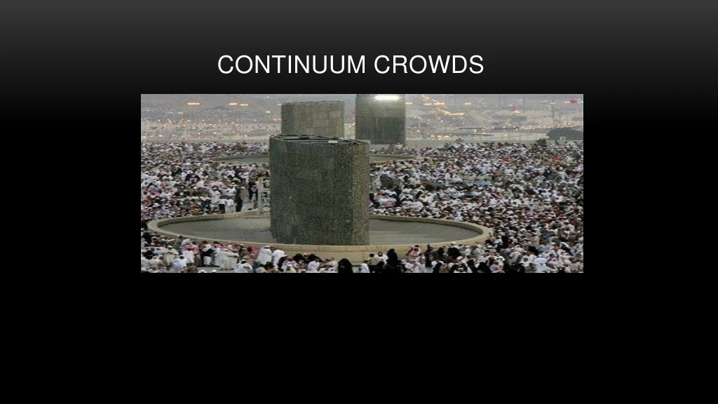
The Flow of Human Crowds - Hughes, 2003 • When? • Characteristic distance scale between pedestrians is less than the characteristic distance scale of the region • Governing equations are non linear partial differential equations • Theoretical model • Applied in analysis of the Jamarat Bridge • Different groups of people possible University of North Carolina, Chapel Hill
Governing eQUATIONS • Conservation of pedestrians • Hypothesis 1: Speed is a function of density and behavioral characteristics • Hypothesis 2: Decisions based on potential which is measured by remaining time • Hypothesis 3: Pedestrians aim to minimize travel time & avoid extreme densities Density ρ, Speed field f, Discomfort field g, Potential Function ϕ, Velocity Components u,v University of North Carolina, Chapel Hill
Applications: Jammarat Bridge University of North Carolina, Chapel Hill
Continuum Crowds – Treuille, et. al., 2006 • Directly inspired by Hughes’ model • Uses concept of particle representation • Similar concepts of potential field and discomfort fields • Individual speed is a function of crowd flow in addition to density • Optimal path takes into account distance • Cost depends on grid size University of North Carolina, Chapel Hill
Hypothesis • Hypothesis 1: Each person is trying to reach a geographic goal G(x,y) • Hypothesis 2: People move at the maximum speed possible, considering environmental conditions f is the maximum speed field (x,), is a unit vector in & is the velocity • Hypothesis 3: There exists a discomfort field g so that, all things being equal, people would prefer to be at point x rather than x’ if g(x’)>g(x) Notation: G(x,y) defines the goal pt. and g(x,y) refers to the discomfort field University of North Carolina, Chapel Hill
Cost Function • People choose paths so as to minimize a linear combination of: • Length of the path • Amount of time to the destination • Discomfort felt, per unit time, along the path • Let C be the unit cost field such that • Notation: • P denotes the path, f the speed field and g is the discomfort field. • ds implies the derivate is w.r.t. distance, dt implies the derivative is w.r.t. time. • , , are weights for the three terms University of North Carolina, Chapel Hill
Optimal Path Computation • Potential Field, • Denotes the cost of the optimal path to the goal for given point • Satisfies the equation: • So velocity at any given point can be computed as • Reducing Computation Cost • Cluster individuals having identical speed field, discomfort and goal into groups • At each timestep, construct a potential field for each group • This is the slowest step of the simulation • Notation: • Potential field • speed field f • C is the unit cost evaluated in the direction of University of North Carolina, Chapel Hill
Density and Velocity Fields • Crowd density field. Ρ • Let ρi denote the density field of the ith function • Average Velocity field • Indicates the overall speed and direction of crowd flow • Notation: • Crowd Density • Average Velocity Field • and denote the density and the velocity of the ith agent resp. University of North Carolina, Chapel Hill
Speed Field • Differs from Hughes Model • Speed field f() measures the maximum permissible speed of movement for every point and every direction in the domain. • If ρ≤ρmin, f = • If ρ> ρmax, f = • Else, linearly interpolate between and • Notation: • is the slope of the height field h in direction . • Position x • Offset r • Density ρ • Topographical Speed • Flow Speed • denote the max. and min. slope University of North Carolina, Chapel Hill
Implementation • For each timestep • Convert the crowd to a density field • Also compute the average velocity field • For each group • Construct the unit cost field C • Compute the maximum speed field f • Construct the potential and its gradient • Update locations • Enforce minimum distance between people University of North Carolina, Chapel Hill
1. Density Conversion • Requirements • Density field must be continuous • Each person should contribute no less than to their own grid cell and no more than to any neighboring grid cell • Density Contribution for each person • ρA=min(1-∆x,1-∆y)λ • ρB=min(∆x,1- ∆y)λ • ρC=min(∆x, ∆y)λ • ρD=min(1-∆x, ∆y)λ • =1/2λ • Simultaneously calculate average velocity field Notation: is the density exponent and is the density University of North Carolina, Chapel Hill
2. Unit Cost Field • Compute maximum speed field f • Compute Cost using f • Keep in mind they are anisotropic • Anticipate obstructions ahead • Notation: • Discomfort field g • Potential field • Density ρ • Height field h • Average Velocity field • Velocity v • Speed field f • Unit cost C University of North Carolina, Chapel Hill
3. Dynamic Potential Field Construction • Fast Marching Method • Cells grouped as KNOWN, UNKNOWN and CANDIDATE • Initially Populate the KNOWN list with goal cells • Loop Until UNKNOWN list is empty • Estimate potential at CANDIDATE cells using finite difference approximation • Add the CANDIDATE cell with the lowest potential to the list of KNOWN cells and its adjacent ‘unknown’ cells to the CANDIDATE list • Running time : O(NlogN) University of North Carolina, Chapel Hill
4. Update Locations • We now have potential field , its gradient and the speed field f • Each persons position is displaced by their velocity • Minimum Distance Enforcement • All fields dependent on resolution of grid • Enforce pedestrians to maintain minimum distance from each other • Simple and Linear in complexity • Introduces artifacts University of North Carolina, Chapel Hill
https://www.youtube.com/watch?v=lGOvYyJ6r1c University of North Carolina, Chapel Hill
Advantages • Unifies global planning and local collision avoidance • Smoother motion • Accounts for crowd flows and includes distance in cost function • Capable of being integrated with agents • Results close to actual observations of large crowds DISADVANTAGES • Not designed for very high density scenarios • Does not take into account uncertainty • People can change direction without respect to inertia • Uniform Grids • Does not have the flexibility and individual variability of the agent-based approach University of North Carolina, Chapel Hill
Aggregate Dynamics for Dense Crowd Simulation - Narain et. al. • Focusses on simulating inter-agent dynamics of large, dense crowds • Combines a Lagrangian representation of individuals with a coarser Eulerian crowd model • Decouples the computational cost of local planning from the number of agents • Overcomes Treuille’s incapability to prevent intersections in very dense crowds University of North Carolina, Chapel Hill
Discrete & Continuous Crowds • Does not combine global and local planners • Augments a continuous representation • Solves for collision avoidance in continuous domain using a variational constraint on the crowd flow, called Unilateral Incompressibility Constraint (UIC). University of North Carolina, Chapel Hill
Agents & the Grid • Accumulate the values carried by nearby agents, weighted by the bilinear interpolation weights • Thus, the crowd is converted to a continuous representation • Notation: • Density • Velocity • and denote the position, pref. velocity and mass of the ith agent • () denote the bilinear interpolation weights associated with agent at position University of North Carolina, Chapel Hill
Unilateral incompressibility constraint (UIC) • Crowd is unlike any physical fluid i.e. it should be treated as a hybrid of purely compressible and purely incompressible • Impose UIC - an inequality constraint Where 1 • Determining corrected velocity v subject to UIC Assume that the agents will try to make as much progress in their desired direction as possible For some scalar “pressure” p>=0 satisfying: University of North Carolina, Chapel Hill
Agent Motion • We now have a flow field through v & which prevents inter agent collision • In dense regions, use continuum velocity • v=v(xi) • In low density regions, interpolate between continuum velocity and agents preferred velocity • Enforce minimum distances for each pair of individual agents University of North Carolina, Chapel Hill
Algorithm • At the beginning of each time step • Global planning is performed to determine the preferred velocity of each agent • The agent positions x and preferred velocities are transferred to the simulation grid • If there are moving obstacles in the environment, the free area of each grid cell is recomputed. • The UIC solve is performed, giving the corrected velocity field v. • Each agent determines its actual velocity taking the corrected flow and updates its position for the next timestep as x = x + t. • Finally, pairwise collision resolution is performed on the new x to handle inter-agent collisions. University of North Carolina, Chapel Hill
Performance University of North Carolina, Chapel Hill
Drawbacks • Pressure projection only looks at local information • No discomfort field i.e. assumption that people aim to maximize progress in the desired direction. • Not as detailed as a purely agent based model University of North Carolina, Chapel Hill
sUMMARY • The Flow of Human Crowds – Hughes et. al. , 2003 • Unifies global and local path planning • Purely theoretical • Time based potential function and density based discomfort and speed field • Continuum Crowds - Treuille et. al. , 2006 • Adapts Hughes’s model for simulation • Potential function based on distance in addition to time and discomfort • Discomfort field can be arbitrarily defined • Speed depends on crowd flow in dense conditions • Aggregate Dynamics for Dense Crowd Simulation - Narain et. al., 2009 • Congestion avoidance on a aggregate level • Separate global and local planners • No notion of discomfort field
References • HUGHES, R. L. 2002. A continuum theory for the flow of pedestrians. Transportation Research Part B 36, 6 (july), 507535. • HUGHES, R. L. 2003. The flow of human crowds. Annu. Rev. Fluid Mech. 35, 169–182. • Treuille, A. Cooper, S. Popović, Z., Continuum Crowds, ACM Transactions on Graphics 25(3) (SIGGRAPH 2006) • Rahul Narain, AbhinavGolas, Sean Curtis, and Ming C. Lin, 2009. Aggregate Dynamics for Dense Crowd Simulation. In ACM Transactions on Graphics (Proceedings of SIGGRAPH Asia), vol. 28, no. 5, pp. 122:1–122:8. • Abhinav Golas, Rahul Narain, and Ming C. Lin, 2013. Hybrid Long-Range Collision Avoidance for Crowd Simulation. In ACM SIGGRAPH Symposium on Interactive 3D Graphics and Games (I3D) 2013. University of North Carolina, Chapel Hill