Download
1 / 25
250 likes | 338 Views
Learn how statistical methods quantify when to end metal loss inspection, predict potential failures, and plan re-inspections. Enhance decision-making with Probability of Exceedance Analysis.

E N D
How do we figure out when to stop digging and when to run the next metal loss in-line inspection. Using statistical methods to help quantify “DONE” R. Turley - MAPL
Let’s start with a small dose of reality • We DON’T normally excavate everything an in-line inspection tool identifies (we leave stuff). • We typically excavate only 5-10% of the metal loss indications an ILI tool identifies. • If you can excavate all anomalies the tool identifies, consider yourself lucky but maybe not as smart as you think. • Everyone defines “DONE” differently • You need different tools with older, pre-CP systems (195,000 anomalies in 110 miles is a lot)
The Challenge • Can we define “done” in a consistent manner so that everyone understands “where” we stopped on a particular line and the level of risk we accept when we do stop? • Can we find a way to quantify our level of “comfort” regarding what we didn’t dig up? • Can we come up with something more justified than a “one-size fits-all” interval?
What information does a metal loss in-line inspection tool provide? • Predicted length of the anomaly • Predicted depth of the anomaly • from this information we can calculate the following for each anomaly: • a Predicted Burst Pressure (Pburst) • a Calculated Allowable Operating Pressure (CAOP) • We can then look at the number of excavations it will take to reach certain criteria.
The Dilemma • In the past, we picked a criteria and dug to it. Refer to previous graphs. • BUT, an in-line inspection tool isn’t perfect. • Typical stated tolerance (for ERW pipe): • +/- 10%, 80% of the time • +/- 15%, 95% of the time • It’s worse for Seamless (+/- 20%, 80% of the time) • So, the question becomes, “if the tool isn’t perfect, how confident are we that we didn’t leave something behind that is a problem.
Using statistics to assist in our decision making • Based on either the tool vendors stated accuracy or our excavation data, we can develop statistical relationships to provide a quantitative way to measure our confidence in a pig’s predicted value. • The “tool” we utilize is a technique known as “Probability of Exceedance Analsysis” or “POE”. • Working on the utilization of this technique for almost three years.
Probability of Exceedance Analysis • Is just a different look at the same data (we just are trying to allow for the tool’s tolerances). • Allows the prioritization of anomalies or groups of anomalies with the greatest probability of causing a release by either a rupture or a leak. • Allows the pipeline mileage to be prioritized by likelihood of a rupture/leak • Demonstrates the impact of a dig program to reduce the likelihood of a corrosion release via either a rupture or a leak.
Probability of Exceedance Analysis • Helps with designing a multiyear dig program and planning reinspection intervals • Allows the potential for adding consequence information and calculating “risk of a leak/rupture due to metal loss.
Ok, what does it all mean? • Now, for each anomaly, we can calculate the potential for the actual value of an un-excavated anomaly to “exceed” a threshold that we identify. • The thresholds we are typically interested in are: • the anomaly is actually deeper than 80% (these anomalies, if they failed, would fail as a leak) • the anomaly has a predicted burst pressure less than the abnormal operating pressure (these anomalies, if they failed, would fail as a rupture) • the anomaly has a CAOP less than MOP
Yeah, so what? • Now, we can quantify the chance or probability that what we didn’t dig could actually be “un-acceptable” • We can correlate our “gut-based” criteria of the past with a quantitative value. • Note, it isn’t truly the chance we are going to have a leak or a rupture, just that our designated threshold is exceeded. It’s the chance the plane has a missing bolt, not that the missing bolt will bring down the plane.
We can now quantify “done” and communicate the relative likelihood of a problem being un-excavated. • We can also treat the risk of a potential burst/rupture failure different than the risk of a potential leak and excavate to different criteria. • We can show the relative reduction in the likelihood of a theoretical leak/rupture with additional excavations. • We can also look at all of our pipeline systems at one time and utilize the information to rank them on a relative basis.
Now what about re-inspection intervals? • Once we can quantify where we stopped, for those anomalies that we leave un-excavated, we model the anomaly with a corrosion growth rate. • When the anomaly grows (in the future) to a certain threshold that we deem in-appropriate (probability of a problem), it’s time to re-inspect. • Just trying to determine broad band justification of the pigging intervals (3-5 yrs, 6-9 years, 10-15 years).
Now the bad news • This only applies to corrosion anomalies (not to 3rd party damage, appurtenances, dents, etc.). • Need different criteria and “gut” reasoning to identify other types of anomalies meriting investigation.
But the good news is…. • All this work confirmed our “gut” feel. • We are doing a much better job of defining and, more importantly, communicating “done”.