Download
1 / 46
460 likes | 599 Views
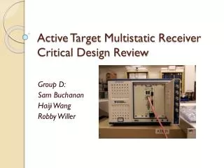
This report presents a comprehensive overview of the multistatic receiver design review led by the team comprising Sam Buchanan, Haiji Wang, and Robby Willer. It includes updates on antenna data gain, received power comparisons, and modifications to the receiver board. The document details the RF functional schematics, parallel convolution processes, and challenges associated with FPGA applications. Also included are clock synthesizer schematics, an integrated test plan, and risk assessments with proposed mitigations to ensure successful demonstration of the ATMR system.

E N D
Active Target MultistaticReceiverCritical Design Review Group D: Sam Buchanan Haiji Wang Robby Willer
Link Budget Update – Antenna Data Gain of airborne antenna array Simulated ATMR antenna gain
FPGA Application (Sequential) 1 2 4 3 1 2 Key steps: Move to baseband (mix with NCO) Decimation Matched filtering Delays for data timing/triggering
Digitization • Parallelization built into NI 5772 • Time interleaved sampling (TIS)
NCO • Implement with Xilinx DDS compiler • 8 NCOs with different phase offsets • Calculate equivalent NCO phase increment
LPF + Downsample • Task: convolution in parallel • Subconvolutions on each channel, sum to produce coherent output
Parallel Convolution Params: fs=1.6 GHz, f0=150MHz, f1=450MHz, t1=10us, p=8, d=4
Parallel Convolution Params: fs=1.6 GHz, f0=150MHz, f1=450MHz, t1=10us, p=8, d=4
Matched Filtering • Correlation filter • Use only the beginning of the LFM waveform as filter coefficients • Use parallel convolution as with LPF
Matched Filtering • Complication: 4 correlators needed (filter coefficients complex) • FPGA only has 288 MACs available • Longer matched filter equates to greater processing gain (RFI resistance) • 64 tap matched filter -> 256 MACs • Only 38 available for LPF stage and other adders • Plan: Implement ATMR with shorter matched filter (32 taps) for demonstration
Delays and Data Transfer • Transfer data to host in 64 bit unsigned quad blocks (16 bit samples) • Challenge: interleaving data properly
Updated Risks • Complexity of FPGA application • Mitigation: work less on host software, more on FPGA • Lack of DSP resources on FPGA • Mitigation: arrange for a new FPGA to be ordered for deployment; plan to demonstrate with shorter filters
Power Analysis • 20 dBm output power
Integrated Test Plan • Work with Dr. Paden to develop test plan • The anechoic chamber has been reserved for testing on May 5-6. • The 1UDAQ will function as the waveform generator for this testing.
Parallel Convolution • Parallel convolution algorithm • Partition LPF impulse response into 8 subsequences • Convolve each impulse response subsequence with each data channel • Symmetry between the decimation factor and number of channels could reduce the number of subconvolutionsequences required to generate coherent output • 8 channels * 8 IR subsequences = 64 total • Sum output using constraints specified in a theorem for reconstruction
Parallel Convolution Example • x = (1, 2, 3, 4); h = (1, 2, 3, 4) • (Example taken from http://ieeexplore.ieee.org/stamp/stamp.jsp?arnumber=00363597&tag=1)
Parallel Convolution Example • 2 parallel channels (p = 2)
Parallel Convolution Example • Compute subconvolution sequences yij (total p2 = 4)
Parallel Convolution Example • To find the nth term of the output y, apply the reconstruction theorem constraints:
Parallel Convolution Example • Apply reconstruction theorem constraints for all values n where y is nonzero • Note: no decimation in this example • If we downsample the output by 2, the only sequences we need are y00 and y11
Parallel Convolution Example • Illustration: downsample y by 2 and re-index n 0 1 2 3 y(n) 1 10 25 16 y00 y00(0) y00(1) y00(2) y11y11(0) y11(1) y11(2)
Parallel Convolution • ATMR has 8 channels, decimates by 3 • Complication: p and the decimation factor are coprime • Need all 64 subconvolutions • Wiring, delays, and timing will be complicated • Implementation plan: keep a state variable, increment and transfer it between executions with a shift register n = 0 1 2 3 4 5 6 7 8 9 10 11 12 13 14 15 16 17 18 19 20 21 22 23 …