Schema-based Program Synthesis and the AutoBayes System
480 likes | 632 Views
Schema-based Program Synthesis and the AutoBayes System. Johann Schumann SGT, NASA Ames. Abstract. This lecture will combine theoretical background of schema based program synthesis with the hands-on study of a powerful, open-source program synthesis system (AutoBayes).

Schema-based Program Synthesis and the AutoBayes System
E N D
Presentation Transcript
Schema-based Program Synthesis and the AutoBayes System Johann Schumann SGT, NASA Ames
Abstract This lecture will combine theoretical background of schema based program synthesis with the hands-on study of a powerful, open-source program synthesis system (AutoBayes). Schema-based program synthesis is a popular approach toward program synthesis. The lecture will provide an introduction into this topic and discuss how this technology can be used to generate customized algorithms. The synthesis of advanced numerical algorithms requires the availability of a powerful symbolic (algebra) system. Its task is to symbolically solve equations, simplify expressions, or to symbolically calculate derivatives (among others) such that the synthesized algorithms become as efficient as possible. We will discuss the use and importance of the symbolic system for synthesis. Any synthesis system is a large and complex piece of code. In this lecture, we will study Autobayes in detail. AutoBayes has been developed at NASA Ames and has been made open source. It takes a compact statistical specification and generates a customized data analysis algorithm (in C/C++) from it. AutoBayes is written in SWI Prolog and many concepts from rewriting, logic, functional, and symbolic programming. We will discuss the system architecture, the schema libary and the extensive support infra-structure. Practical hands-on experiments and exercises will enable the student to get insight into a realistic program synthesis system and provides knowledge to use, modify, and extend Autobayes.
Climate Change... • A recent (end 7/2011) publication in New Scientist: “Raw Data published” • Data contain temperature data from weather stations worldwide since 1850 • and two Perl scripts to preprocess data http://www.metoffice.gov.uk/research/climate/climate-monitoring/land-and-atmosphere/surface-station-records
The Data I • The raw data are in a textual format. • Running script 1 yields grid data (lat*long) for each month • 36x72x12x160 • ASCII file with in-between headers • missing data values = 1e30 • Preparing for analysis:manual editing or scripting magic to get this into octave or Matlab for further analysis • Images show data for different months and years
The Data II • Running script 2 produces averaged (annual) time series • “trend” is easy to recognize, although there is a lot of noise • These are the given data: Can we do more analysis?
Statistical Data Analysis statistical model: the model gives a high level, parameterized description (“specification”) of the data. For example: + • Task: find the unknown parameters that best explain the data, i.e., that most closely fit the data. • Statistics speak: • How: • write a program • use a statistical library • use AutoBayes
Statistical Data Analysis Just a very simple example model. There might be more than one change points
Parameter Estimation I model warming_1. const nat n. where 0 < n. data double temp(0..n-1). const double sq1. where 0 < sq1. const double sq2. where 0 < sq2. double level. double rate. nat t_0. where t_0 < n - 1. where 2 < t_0. where t_0 in 3..n-3. temp(I) ~ gauss( cond(I < t_0, level, level + rate *(I - t_0)), cond(I < t_0, sqrt(sq1), sqrt(sq2)) ). max pr({temp}|{level, rate, t_0}) for {level, rate, t_0}. • we have n data points • before the change point the data are constant (w/noise!), after that they increase linearly • Assume: noise is Gaussian and sigma’s are known (we just guess them here) • Estimate • level • rate • t_0 t_0
Parameter Estimation I demo: run_warming_1 • given noise parameters: 0.3 and 0.2 • How about estimating the noise parameters as well?
Parameter Estimation II max pr({temp}|{level, rise, sq1, sq2, t_0}) for {level, rise, sq1, sq2, t_0}. • same as before, but unknown sq_1, sq_2 • Cannot find a closed form solution: must add pragma to allow generation of iterative approximation • results not good: • sq1 = sq2 =1 pragma schema_control_arbitrary_init_values=true.
Parameter Estimation III model warming_4. const nat n. data double temp(0..n-1). double sq1. where 0 < sq1. double sq2. where 0 < sq2. const nat sigma_1_0. % guess value for the sq_1 where 0 < sigma_1_0. const nat sigma_2_0. % for sq_2 where 0 < sigma_2_0. const double delta_1_0. % confidence level about our prior where 0 < delta_1_0. const double delta_2_0. where 0 < delta_2_0. % definition of the conjugate prior sq1 ~ invgamma(delta_1_0/2+1, sigma_1_0*(delta_1_0/2)). sq2 ~ invgamma(delta_2_0/2+1, sigma_2_0*(delta_2_0/2)). .... rest as usual ... max pr({temp}|{level, rate, sq1, sq2, t_0}) for {level, rate, sq1, sq2, t_0}. • We use “prior” knowledge on the noise parameters, i.e., we have an “idea” how large the sigmas are • “conjugate prior” is the form the statistician would use here • generates single-variable iterative algorithm
Parameter Estimation III • Priors allow to model “soft” constraints on model parameters l = -0.30740 r = 0.013809 s1 = 0.16667 s2 = 0.0083333 t0 = 1850+ 96 with: s1_0 = 1 s2_0 = 0.05 delta = 0.8
Experience • Data available and relatively easy to convert to octave format • initial models set up within a few minutes; getting the data into the right format was more difficult (-> synthesis opportunity) • easy to “explore” different models and parameters much quicker than direct programming • AutoBayes currently does not handle hard constraints very well • Which model is the “right” one? • AutoBayes cannot iterate over different models and find the one that best fits the data • One could specify a generator for the model structure: one change point, more change points, etc. (sketch-like, perhaps)
More Data Analysis 36x72 • Let’s find some structure in the data cube. • Are the sequences of data readings somehow related between the stations? • Can they reveal some structure? E.g., particularly strong warming, same cooling periods, ... • Clustering is an unsupervised machine learning technique that tries to find structure in the data 1920=160x12 time
Example: Simple Clustering • Given: data-points that originate from 3 different sources or “processes” (red, green, blue) • Data points are: • have the same statistical properties • Gaussian distributed Problem: you don’t see the colors
Example: Simple Clustering • Clustering task: Estimate the unknown parameters µ, such that P(x| µ,) is maximal Mmhm–not so easy :-( [an iterative algorithm is needed] Literature says: use k-means or EM algorithm
AutoBayes Specification model mog as ‘mixture of Gaussians. const nat N as ’number of data points'. where 0 < N. const nat C := 3. where 0 < C. where C << N. double µ(0..C-1), (0..C-1). double phi(0..C-1) as 'class frequency'. where 0 = sum(_i := 0 .. C-1, phi(_i))-1. output double c(0..N-1) as ‘class assignment’. c(_) ~ discrete(vector(_i := 0 .. C-1, phi(_i))). data double x(0..N-1). x(_i) ~ gauss(µ_alt(c(_i)), _alt(c(_i))). max pr({x} |{phi, , µ} for {phi, , µ}. • complete AutoBayes specification • domain specific input language “statistician’s speak” • fully declarative What do we synthesize?
AutoBayes Demo • running AutoBayes • generated artifacts: • C++ code for octave (or C for Matlab) • the design document according to NASA standards • specification • input-output code interface • Bayesian graph • additional preconditions • commented code • LaTeX mathematical derivation (later)
Clustering of Climate Data • clustering into 3 groups (classes)
Clustering of Climate Data • clustering into 5 groups (classes)
Clustering of Climate Data • clustering into 7 groups (classes) • the model has to deal with missing data
Another (tiny) example • Measuring the “foot” • The full AutoBayes specification model av_foot. const int n as ‘#measurements’. double mu. double sigma. data double l_foot(0..n_ac-1). l_foot(_) ~ gauss(mu, sigma). max pr(l_foot | {mu, sigma}). • AutoBayes does automatically a first-principle derivation and does not know about: norm.pdf This is the smallest example in the 160+ pages manual
Current AutoBayes Applications IRIS Astronomy science Software Testing Earth Science/Geodata Air Traffic Control
What is AutoBayes? • Customizable Bayesian data analysis code generator • Synthesizes custom algorithms • Generates C/C++ for Matlab, Octave or embedded systems • Generates documentation • Input is statistical model of analysis problem • Looks like a compiler for a very high, domain-specific language SPECIFICATION C/C++ Code
So, What is AutoBayes? • schema-based program synthesis • heavily relies on symbolic system, rewriting, etc. • implemented in SWI Prolog
Prolog • History • constants, terms and variables • matching (and unification) • clauses and their execution • procedural programming • search and backtracking • the global data base • Input/Output • Meta programming
Prolog–History • Colmerauer, 1972 • mainly used for AI, linguistics, semantic web, ... (mainly Europe; USA: Lisp) • roots in first-order logic • prolog execution: SLD resolution • clausal normal form • many extensions toward • constraint logic programming • parallelism • expert systems • ... • several mature implementation available
Prolog–constants, terms, variables • constants and function symbols start with a lowercase letter, e.g., myconst, f(a,b) • lists are [first | rest] or [first, second, third] • Variables start with an Upper case letter, e.g., X, Y, _ (anon. variable) • Terms and variables are untyped • User-defined operators are possible, e.g., max pr(...) for {...} • Examples: • f(X, a, [aa | _], Y) • f(a,b) = .. [ f, a, b]
Prolog–Matching • Prolog’s way of passing parameters is matching of two terms s, t • If s,t match then there is a variable substitution such that sigma s = t • (unification is s = t) • Example: • f(a,g(X, b)) with • g(a,g(X,b)): matching fails. • f(Y,Z): Y=a, Z=g(X,b) • f(a,g(c,b): X = c • first-order matching only: no matching of function symbols, e.g., X(a,b) is not a legal term
Prolog–clauses • A Prolog program is a set of clauses and a query • A clause consists of a head and 0 or more subgoals. • All variables are local to each clause • Example: myprint([]). myprint([F|R]) :- writeln(F), writeln(‘,’), myprint(R). ?-myprint([a,b,c,d]). unit clause (fact) rule with head and subgoals query
Prolog–procedural style • Each clause can seen as a small “procedure”. If the matching with the head succeeds, the subgoals are executed in the given order before the clause “returns” • If the matching fails, the next clause with the same predicate symbol is tried • Recursive calls are used all the time • Variables are used to pass parameters and to return values • Example: length([], 0). length([F|R], L) :- length(R,LR), L is LR + 1. ?- length([a,b,c],L) L=3
Prolog–search & backtrack • Prolog performs a depth-first search with backtracking during the execution. • Whenever a matching with a clause fails, Prolog back-tracks and automatically undoes variable bindings • Powerful programming paradigm, but programming errors can lead to infinite descents or large, hard-to-control search spaces • Cuts (!) can remove parts of the search space, but beware
Prolog–global data base • All variables in Prolog are local to a clause and only live as long as the clause is active • Persistent data can be used with • Flags: • flag(myflag, _, 1). % set to 1 • flag(myflag, X, X), % query flag, result in X • Asserts: • assert(drink(beer)). % puts clause drink(beer) into data base • ?-drink(X) X=beer • These constructs are not backtrackable • NOTE: for AutoBayes, we have implemented special, backtrackable flags (bflag) and asserts (bassert)
Prolog–IO • all sorts of file IO, etc. • you need to know: • write(Term) % writes term to screen • writeln(Term) % with newline
Prolog–Meta Programming • Meta-programming is a very powerful construct in Prolog • Basic predicate: call(P) • calls predicate P • Example: • call(length([a,b,c],X)), writeln(X).
Schema-based Synthesis a’la AutoBayes • a schema is a partial program with holes and applicability constraints • holes filled by • calculations (e.g., solution of an equation) • recursive calls to schemas • code templates and code • We use Prolog clauses to represent schemas and Prolog variables for holes • multiple variants of schemas are explored using Prolog backtracking • advantage: large granularity leads to small search space • disadvantage: does not generate programs from first principle; schema based synthesis is restricted to domain-specific applications.
Schemas & Holes • Sketch: • holes (??) are filled with constants • structure of the “spec” is flexible and generated • UDITA • holes are filled with integer values during runtime • Keplar • holes are filled with pre-compiled integer values • deductive synthesis • quantified variables ( exists P forall I (.....)) • AutoBayes • holes are filled with constants, formulas, or code fragments • symbolic calculation done as far as possible during synth • when no symbolic solution is found: instantiate numeric solver
Schemas & Synthesis • AutoBayes • uses backtracking search w/applicability constraints to generate solution(s) and program(s) • Others • games & strategies • constraint solver • explicit model checking • SAT/SMT • first or higher order theorem prover “proof as program”
Schemas and ... • AB schemas have a coarse granularity • lots of domain knowledge is formalized in schema • schema encapsulates control flow (as opposed to: inductive proof -> recursive program) • no correct-by-construction • see later discussion on AutoCert
Example • Generate a program that finds the maximum value of a function f(x): max f(x) wrt x univariate multivariate Note: the function might be given as a formula or a vector of data
Schema for univariate optimization schema(max F wrt X, C) :- % INPUT (Problem), OUTPUT (Code fragment) % guards length(X, 1), % come up with the solution.. C = ... % recursive schema calls . • All schemas in AB are, in principle, following this syntactic form • in AB, most schemas add some predicates for tracing and debugging
Find the maximum • If the formula is known, the we can do the text-book style technique: 1. build the derivative: df/dx 2. set it to 0: 0 = df/dx 3. solve that equation for x 4. the solution is the desired maximum
Schema for univariate optimization schema(max F wrt X, C) :- % INPUT (Problem), OUTPUT (Code fragment) % guards length(X, 1), % calculate the first derivative simplify(deriv(F, X), DF), % solve the equation solve(true, 0 = DF, X, S), % possibly more checks C = S . . • build the derivative: df/dx • set it to 0: 0 = df/dx • solve that equation for x • the solution is the desired maximum
Schema for univariate optimization schema(max F wrt X, C) :- % INPUT (Problem), OUTPUT (Code fragment) % guards length(X, 1), % calculate the first derivative simplify(deriv(F, X), DF), % solve the equation solve(true, x, 0 = DF, S), % possibly more checks % is that really a maximum? simplify(deriv(DF, X), DDF), solve(true, x, 0 > DDF, _), C = S . . • build the derivative: df/dx • set it to 0: 0 = df/dx • solve that equation for x • the solution is the desired maximum
Schema for univariate optimization schema(max F wrt X, C) :- % INPUT (Problem), OUTPUT (Code fragment) % guards length(X, 1), % calculate the first derivative simplify(deriv(F, X), DF), % solve the equation solve(true, x, 0 = DF, S), % possibly more checks % is that really a maximum? simplify(deriv(DF, X), DDF), (solve(true, x, 0 > DDF, _) -> true ; writeln(‘Proof obligation not solved automatically’) ), C = S . . • build the derivative: df/dx • set it to 0: 0 = df/dx • solve that equation for x • the solution is the desired maximum
Schema for univariate optimization schema(max F wrt X, C) :- % INPUT (Problem), OUTPUT (Code fragment) % guards length(X, 1), % calculate the first derivative simplify(deriv(F, X), DF), % solve the equation solve(true, x, 0 = DF, S), % possibly more checks % is that really a maximum? simplify(deriv(DF, X), DDF), (solve(true, x, 0 > DDF, _) -> true ; writeln(‘Proof obligation not solved automatically’) ), XP = [‘The maximum for‘, expr(F), ‘is calculated ...’], V = pv_fresh, C = let(assign(V, C, [comment(XP)]), V). . . • build the derivative: df/dx • set it to 0: 0 = df/dx • solve that equation for x • the solution is the desired maximum
Schemas for univariate optimization schema(max F wrt X, C) :- ... as before schema(max F wrt X, C) :- length(X, 1), % F is a vector of data points F(0..n) C = let(sequence([ assign(mymax,0), for(idx(I,0,n), if(select(F,I) > mymax, assign(mymax, select(F,I)), skip)... ]), comment([‘The maximum is found by iterating...’]), mymax). schema(max F wrt X, C) :- length(X, 1), % instantiate numeric solution algorithm % e.g., golden section search C = ... schema(max F wrt X, C) :- ... . .