Download
1 / 29
290 likes | 435 Views
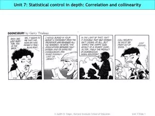
Unit 7: Statistical control in depth: Correlation and collinearity. The S-030 roadmap: Where’s this unit in the big picture?. Unit 1: Introduction to simple linear regression. Unit 2: Correlation and causality. Unit 3: Inference for the regression model. Building a solid foundation.

E N D
Unit 7: Statistical control in depth: Correlation and collinearity
The S-030 roadmap: Where’s this unit in the big picture? Unit 1: Introduction to simple linear regression Unit 2: Correlation and causality Unit 3: Inference for the regression model Building a solid foundation Unit 5: Transformations to achieve linearity Unit 4: Regression assumptions: Evaluating their tenability Mastering the subtleties Adding additional predictors Unit 6: The basics of multiple regression Unit 7: Statistical control in depth: Correlation and collinearity Generalizing to other types of predictors and effects Unit 9: Categorical predictors II: Polychotomies Unit 8: Categorical predictors I: Dichotomies Unit 10: Interaction and quadratic effects Pulling it all together Unit 11: Regression modeling in practice
In this unit, we’re going to learn about… • What is really meant by statistical control? • Is statistical control always possible?: The problem of collinearity • Learning how to examine a correlation matrix and what it foreshadows for multiple regression • Using Venn diagrams to develop your intuition about correlation • Measuring the additional explanatory power of additional predictors • Partial correlation—terminology, interpretation, and relationship to simple correlation • Multiple correlation—its relationship to R2 • Suppressor effects: When statistical control can help reveal an effect • The dangers of multicollinearity: • what it is • how to spot it • what to do about it
When and why is statistical control important? 16 March 1992 Lead, Lies and Data Tape Two psychologists, both of whom have testified for the lead industry and one of whom has received tens of thousands of dollars in research grants from the industry, have filed misconduct charges against the scientist who first linked "low" levels of lead to cognitive problems in children. They don't suspect that Herbert Needleman of the University of Pittsburgh stole, faked or fabricated data. Rather, they say, he selected the data and the statistical model -- the equations for analyzing those data -- that show lead in the worst possible light… The allegations center on a 1979 paper. It describes how Needleman and colleagues measured the lead in baby teeth, looking for a link between lead and intelligence. NIH told Pittsburgh to convene a panel of inquiry. The panel's report, submitted in December and obtained by NEWSWEEK, found that Needleman didn't "fabricate, falsify or plagiarize." It did have problems with how he decided whether or not to include particular children in his analysis, but called this "a result of a lack of scientific rigor rather than the presence of scientific misconduct." The panel found Needleman's statistical model "questionable," though. On that basis, the university launched an investigation. Scarr, Ernhart and the Pittsburgh panel all condemn Needleman for not using a different model -- one that, say, factored in the age of each child. If he had, they say, lead would not have had an impact on IQ. But last year Environmental Protection Agency scientist (and recipient of a MacArthur Foundation "genius" award) Joel Schwartz reanalyzed Needleman's data. He factored in age explicitly. "I found essentially the identical results," he says. • Randomized experiments: Statistical control is not as crucial • Researcher actively intervenes in the system observing how changes in X produce changes in Y • Random assignment ensures that, on average, treated and control groups are equivalent on all observed and, even more importantly, unobserved variables • Even so, statistical control still helps as it increases the precision of our estimates • Observational studies, sample surveys and quasi experiments: Statistical control is much more important • With no active external intervention, individuals effectively “choose” their own values of X • Individuals with particular values of X may differ on observed variables—this is when statistical control can help • More problematic is when individuals with particular values of X may also differ on unobserved variables—then you need statistical methods that are more advanced than we cover in S-030
How statistical control can help, Example I: Cross sectional study examining predictors of reading scores in elementary school Taller children have higher reading scores 6 5 READING 4 3 2 1 HEIGHT There’s no statistically significant relationship between reading scores and height Older students read better (duh) Main Effects Model Do we really believe this or is there a 3rd variable for which we should statistically control? GRADE Main effect: we’ve assumed the effect to be the same across all grades = parallel lines Controlling for a predictor can stop us from concluding (erroneously) that a spurious correlation is real
How statistical control can help, Example II: Does the availability of guns save lives (or kill people?) Communities with more gun licenses have lower violent crime rates VIOLENT CRIME RAE # GUN LICENSES There’s now a positive relationship between Gun Licenses and the violent crime rate (the sign of the estimated regression coefficient is reversed!) The more urban the community, the higher the violent crime rate Urbanicity Do we really believe this or is there a 3rd variable for which we should statistically control? Very urban Very rural Controlling for a predictor can reveal or reverse the direction of an effect
How statistical control should be able to help (but sometimes can’t!) Sex discrimination in clerical salaries at Yale On average, women have lower wages than men On average, women are in lower status jobs than men Wages Job Status There’s no statistically significant wage differential between men and women controlling for job status Higher status jobs pay more Can we really control statistically for the effects of job status and really evaluate the effects of gender? Men Women If predictors are “too highly” correlated with each other, we can’t statistically control for the effect of one and evaluate the effects the other: This is known as (multi)collinearity
Two new predictors for USNews: Research Funding & Pct Doc Students HGSE HGSE Stanford Stanford Peer Ratings of US Graduate schools of education Peer Res Pct ID School Rat GRE L2Doc Fund Doc 1 Harvard 450 6.625 5.90689 17.4 35.8 2 UCLA 410 5.780 5.72792 36.4 46.8 3 Stanford 470 6.775 5.24793 15.1 48.0 4 TC 440 6.045 7.59246 30.1 37.5 5 Vanderbilt 430 6.605 4.45943 23.0 48.6 6 Northwestern 390 6.770 3.32193 8.8 47.0 7 Berkeley 440 6.050 5.42626 12.0 56.3 8 Penn 380 6.040 5.93074 19.0 41.0 9 Michigan 430 6.090 5.24793 19.0 62.7 10 Madison 430 5.800 6.72792 25.5 53.8 . . . • RQ: Does research production predict variation in the peer ratings of GSEs? • Total Research $ • Pct Doctoral Students Predictor: ResFund Mean 11.29540 Std Dev 8.13018 Stem Leaf # Boxplot 36 4 1 0 34 32 30 14 2 | 28 | 26 4 1 | 24 5158 4 | 22 08 2 | 20 13 2 | 18 14002 5 | 16 145671479 9 +-----+ 14 112 3 | | 12 068826 6 | | 10 125715679 9 *--+--* 8 5580458 7 | | 6 0256828 7 | | 4 11172356778 11 +-----+ 2 1158891237 10 | 0 33667056 8 | Predictor: PctDoc Mean 38.1965517 Std Dev 16.3568807 Stem Leaf # Boxplot 9 1 1 0 8 8 0 1 0 7 7 1 | 7 | 6 9 1 | 6 2333 4 | 5 5668 4 | 5 0033444 7 | 4 567777889 9 +-----+ 4 01133 5 | | 3 566666778888888888999 21 *--+--* 3 011114 6 | | 2 555567899999 12 +-----+ 2 14 2 | 1 56778889 8 | 1 44 2 | 0 567 3 | Claremont UCLA UC Riverside TC, NYU USC Penn State
Relationship between Peer Ratings and the two new predictors The REG Procedure Dependent Variable: PeerRat Sum of Mean Source DF Squares Square F Value Pr > F Model 1 42509 42509 27.24 <.0001 Error 85 132664 1560.74781 Corrected Total 86 175172 Root MSE 39.50630 R-Square 0.2427 Dependent Mean 344.82759 Adj R-Sq 0.2338 Coeff Var 11.45683 Parameter Standard Variable DF Estimate Error t Value Pr > |t| Intercept 1 313.93941 7.27801 43.14 <.0001 ResFund 1 2.73458 0.52398 5.22 <.0001 The REG Procedure Dependent Variable: PeerRat Sum of Mean Source DF Squares Square F Value Pr > F Model 1 38775 38775 24.16 <.0001 Error 85 136397 1604.67212 Corrected Total 86 175172 Root MSE 40.05836 R-Square 0.2214 Dependent Mean 344.82759 Adj R-Sq 0.2122 Coeff Var 11.61692 Parameter Standard Variable DF Estimate Error t Value Pr > |t| Intercept 1 295.24240 10.96333 26.93 <.0001 PctDoc 1 1.29816 0.26408 4.92 <.0001 Stanford Stanford HGSE HGSE
Examining the correlation matrix, Step 1: Get output (using PROC CORR) Describes cell entries (r and p-value, all with N=87) Notice the symmetry Pearson Correlation Coefficients, N = 87 Prob > |r| under H0: Rho=0 (H0: =0) PeerRat L2Doc GRE ResFund PctDoc PeerRat 1.00000 0.46393 0.65654 0.49261 0.47048 <.0001 <.0001 <.0001 <.0001 L2Doc 0.46393 1.00000 0.14528 0.51096 0.31777 <.0001 0.1794 <.0001 0.0027 GRE 0.65654 0.14528 1.00000 0.40573 0.17045 <.0001 0.1794 <.0001 0.1145 ResFund 0.49261 0.51096 0.40573 1.00000 0.05695 <.0001 <.0001 <.0001 0.6003 PctDoc 0.47048 0.31777 0.17045 0.05695 1.00000 <.0001 0.0027 0.1145 0.6003 Always list the outcome first so the table is easiest to read Like most computer output, it provides “too much detail” r = 0.32** r = 0.17 (ns) 2 decimal places and *’s usually suffice * p<0.05, ** p<0.01, *** p<0.001
Examining the correlation matrix, Step 2: Create a summary table The correlation between our two original predictors—GRE and L2Doc—is not statistically significant Research funding is significantly correlated (p<0.001) with both program size and mean GRE scores The percentage of doctoral students is significantly correlated (p<0.01) with the log(# of doctoral students), but not with either mean GRE or Research Funding The correlation between each predictor and Peer Ratings is statistically significant (p<0.001). We already knew this on the basis of the simple linear regressions, but typically, we’d estimate these correlations before looking at those regression results What do these correlations foreshadow for multiple regression? The information in research funding may be redundant with other variables already in the model, but the information in PctDoc may explain additional variation in Peer Ratings
A visual inspection of correlations: PeerRat vs. each predictor r = 0.66 r = 0.46 r = 0.49 r = 0.47
The scatterplot matrix: A graphic correlation matrix .46 .66 .49 .47 .15 .51 .32 .41 .17 .06
Questions we can ask about correlations between variables:How Venn diagrams can help us understand complex interrelationships • Our learning goal: To understand the interrelationships among the correlations • How much variation in Y is explained by X1 and X2 together • How much variation in Y is explained by X1 after controlling for X2 • How much variation in Y is explained by X2 after controlling for X1 • One outcome (Y) and 2 predictors (X1 and X2)—generate 3 correlations to examine: • Correlation between each predictor and Y: rY1 and rY2 • Correlation between the two predictors: r12 Y Y X1 X2 X1 X2
Contrasting Venn diagrams with uncorrelated and correlated predictors R2 predicting Y using only X1 R2 predicting Y using only X2: Y Y X1 X2 b a a b c c X1 X2 Uncorrelated predictors Uncorrelated predictors are very rare, arising mostly in designed experiments. We can compute the overall R2 by just summing the separate R2’s Correlated predictors Correlated predictors are very common, arising in almost all studies. We can’t just sum the separate R2 statistics because of the overlap Y Y X1 X2 b a X1 X2 c • How do correlations between predictors affect their joint utility? • Highly correlated predictors: Jointly explained portion “c” is large; Additional independent portions “a” and “b” are small • Fairly uncorrelated predictors: Jointly explained portion “c” is small; additional independent portions “a” and “b” are large
Measuring the additional explanatory power of an additional predictor How are partials related to simple correlations? Partial Correlation2 Simple Correlation2 Assuming that X1 is already in the model, how can we measure X2’s additional contribution, over and above that already explained by X1? Y d X1 X2 b a c • Clarifying terminology and notation • Simple correlation, rY2 and RY|22 : Proportion of variation in Y associated with X2 • Multiple correlation, RY|122: Proportion of variation in Y associated with both X1 and X2 • Partial correlation, rY2|1 : Y2 identifies the variables being correlated; |1 identifies the variable(s) being controlled (or partialled out) Comparing these 2 equations, we see that b & d are in both denominators. So the relationship between simples and partials depends upon the size of “a” & “c” relative to “b” & “d”
Understanding the relationship between partial and simple correlations Partials can equal simples Partials can be greater than simples Partials can be smaller than simples Y Y Y a d d d c b b a b c X1 X2 X2 X1 X1 X2 When “a” and “c” are small: Simple Partial When “a” is large (and “c” is large or small): Partial > Simple When “c” is large (and “a” isn’t very large): Partial < Simple a c Most common reason: X1 is relatively uncorrelated with Y Most common reason: X1 is very highly correlated with Y Most common reason: X1 is very highly correlated with X2
Partial correlations for the USNews data, controlling for L2Doc Major decision: Which variable(s), if any, should we partial out? Describes cell entries (r and p-value, all with N=87) Again, notice the symmetry Pearson PartialCorrelation Coefficients, N = 87 Prob > |r| under H0: Rho=0 PeerRat GRE ResFund PctDoc PeerRat 1.00000 0.67217 0.33561 0.38461 <.0001 0.0016 0.0003 GRE 0.67217 1.00000 0.38978 0.13249 <.0001 0.0002 0.2240 ResFund 0.33561 0.38978 1.00000 -0.12934 0.0016 0.0002 0.2353 PctDoc 0.38461 0.13249 -0.12934 1.00000 0.0003 0.2240 0.2353 Continue to list the outcome first so the table is easiest to read Like most computer output, it provides “too much detail” Go to simple correlation output
Understanding the link between partial correlations and MR Partial correlations quantify the association between two variables after controlling statistically for one (or more) predictors Multiple regression models quantify the association between two variables after controlling statistically for one (or more) predictors ??????? Parameter Standard Variable DF Estimate Error t Value Pr > |t| Intercept 1 -87.29494 43.07364 -2.03 0.0459 L2Doc 1 15.34201 2.94746 5.21 <.0001 GRE 1 63.31660 7.60956 8.32 <.0001 PartialCorrelation Coefficients controlling for L2Doc PeerRat GRE ResFund PeerRat 1.00000 0.67217 0.33561 <.0001 0.0016 GRE 0.67217 1.00000 0.38978 <.0001 0.0002 ResFund 0.33561 0.38978 1.00000 0.0016 0.0002 PctDoc 0.38461 0.13249 -0.12934 0.0003 0.2240 0.2353 Parameter Standard Variable DF Estimate Error t Value Pr > |t| Intercept 1 262.96680 20.06665 13.10 <.0001 L2Doc 1 11.70357 4.31624 2.71 0.0081 ResFund 1 1.91994 0.58799 3.27 0.0016 Parameter Standard Variable DF Estimate Error t Value Pr > |t| Intercept 1 233.68011 19.46286 12.01 <.0001 L2Doc 1 14.25165 3.83448 3.72 0.0004 PctDoc 1 0.99151 0.25964 3.82 0.0003 Partial correlations and multiple regression are intimately linked The p-value for the partial correlation between Y and a predictor, say X2, after controlling statistically for other predictors, say just X1, is identical to the p-value for the slope coefficient for X2 in a multiple regression model that includes both X2 and X1
Comparing simple and partial correlations for the USNews data The partial correlation with mean GRE is virtually unchanged while the partial correlations with Research Funding and PctDoc students decline (but are still stat sig.) [This makes sense because Log2(N doc grads) was virtually uncorrelated with mean GRE, but was significantly correlated with Research Funding and PctDoc students.] Research Funding remains correlated with Mean GRE after controlling for program size PctDoc Peer L2Doc GRE ResFund PctDoc students remains uncorrelated with the other predictors, even after controlling for program size
Results of fitting additional MR models to USNews data Some things to consider when selecting models to present • Does the model chosen reflect your underlying theory? • Does the model allow you to address the effects of your key question predictor(s)? • Are you unnecessarily including predictors you could reasonably set aside (the parsimonyprinciple)? • Are you excluding predictors that are statistically significant [If so, why exclude them?] • Always realize that NO model is ever “final” • We’ll spend much, much, much more time on this topic in Unit 11
Is it always possible to statistically control? • Our language for MR has used many terms for statistical control: • Controlling for X1 • Holding X1constant • Removing the effects of X1 • This language assumes that we can really hold X1 constant and X2 will still vary across its full range, but is this always true? • Now: What happens if holding X1 constant dramatically restricts the range in X2—can we really statistically control for one predictor and evaluate the effects of another? Aver educ • Example: National Child Care Survey • n = 45 two parent Latino families • RQ: What is the relationship between parental education and family income? • Two parental education predictors:Mother’s and father’s education Go to: Multicollinearity: What it is, why it happens, how to spot it, and what to do
Multicollinearity: What it is, why it happens, how to spot it, and what to do MomEd DadEd • What is multicollinearity? When two (or more) predictors are so highly correlated that we cannot statistically control for one predictor and evaluate the effect of the other(s) • Mother’s & father’s education • Gender and job status at Yale • Family background & school resources Income d a b c • How to spot multicollinearity • Controlled & uncontrolled slopes differ dramatically for two (or more) predictors • The estimated controlled slopes make no sense (e.g., the signs appear wrong!) • Standard errors increase with added predictors • Reject omnibus F test but fail to reject individual t-tests for the constituent predictors • What to do about multicollinearity • Use better research designs—especially randomized trials—that eliminate confounding • Collect more data, especially “unusual cases” • Collapse collinear predictors into a composite • Include just one of the collinear predictors in your MR model (but be sure to explain what you did and why you did it) What happens when we create a composite—Average Education —for the NCCS data?
Caution: Don’t assume that all strongly correlated predictors are collinear 6 5 4 3 2 1 READING Partialling out Height, there’s still an effect of Grade Reading Partialling out Grade, there’s virtually no effect of Height HEIGHT Grade Height Conclusion: Height and grade are strongly correlated, but not collinear Don’t abuse the phrase… Holding Height constant, however, there is still variation in Grade, and that variation is associated with Reading d b a c
Coda: Sometimes the direction of an effect can change upon statistical control!Suppressor effects in predicting faculty salaries at the University of Kansas Salary $100,000 $80,000 $60,000 0 5 10 15 20 Years of Service at University “Salary compression…the failure of the organization to recognize seniority with adequate compensation increase while meeting current market values for lower ranked individuals hired into the institution” McCulley & Downey (1993) Salary compression in faculty salaries: Identification of a supressor effect. Educational and Psychological Measurement, 53, 79-86 • Higher ranked professors have higher salaries • Department heads have higher salaries • Higher ranked professors are more likely to be department heads • The more years of service, the higher the rank 10,493 Full Professor Dept Head 15,905 Assoc Professor 15,905 10,493 Full Professor Not Dept Head 10,493 Assoc Professor • But there are two very surprising findings concerning Years of Service: • No correlation between years of service and salary? • No correlation between years of service and being a department head? Asst Professor R2 = 65%
Start looking at the results sections of papers in your substantive fields… Michal Kurlaender & John Yun (2007) Measuring school racial composition and student outcomes in a multiracial society, American Journal of Education, 113, 213-242
Another example of presenting regression results in journals Barbara Pan, Meredith Rowe, Judith Singer and Catherine Snow (2005) Maternal correlates of growth in toddler vocabulary production in low-income families, Child Development, 76(4) 763-782
What’s the big takeaway from this unit? • Statistical control is a very powerful tool • The ability to statistically control for the effects of some predictors when evaluating the effects of other predictors greatly expands the utility of statistical models • It allows you to acknowledge the effects of some predictors and then put all individuals on a “level playing field” that holds those controlled predictors constant • The pattern of correlations can help presage multiple regression results • Learn how to examine a correlation matrix and foreshadow how the predictors will behave in a multiple regression model • If you have one (or more) control predictors, consider examining a partial correlation matrix that removes that effect • Controlled effects can be similar to or different from uncontrolled effects • The effects of some predictors will persist upon statistical control while the effects of others will change • Be sure to examine how your predictors effects change as you fit more complex statistical models • Ask yourself whether the observed changes make sense • Beware of the dangers of multicollinearity • Sometimes it isn’t possible to statistically control • When your predictors are highly correlated, you may think you’re statistically controlling for the effects of one when you’re evaluating the effects of the other, but this may not be possible • But similarly, just because predictors are highly correlated, don’t assume that you’ll have collinearity problems
Appendix: Annotated PC-SAS Code for Estimating Partial Correlations proc correstimates simple correlations between the variables specified. Its var statement syntax is var1 var2 var3 … varn. proc corr data=one; var PeerRat L2Doc GRE ResFund PctDoc; proc corr data=one; partial l2doc; var PeerRat GRE ResFund PctDoc; proc corr can also estimate partial correlations. Use a partial statement to identify the variable(s) being controlled (partialled out). Note that the handouts include only annotations for the needed additional code. For the complete program, check program “Unit 7—Statistical Control in Depth” on the website. Note also that this annotation builds on the knowledge from “Unit 2 – Correlation and Causality”. • Correlation • Cross-sectional data • Main effects assumption/model • Multicollinearity • Statistical control Glossary terms included in Unit 7