Project Objectives
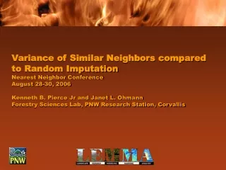
Variance of Similar Neighbors compared to Random Imputation Nearest Neighbor Conference August 28-30, 2006 Kenneth B. Pierce Jr and Janet L. Ohmann Forestry Sciences Lab, PNW Research Station, Corvallis. Project Objectives.

Project Objectives
E N D
Presentation Transcript
Variance of Similar Neighbors compared to Random ImputationNearest Neighbor ConferenceAugust 28-30, 2006Kenneth B. Pierce Jr and Janet L. OhmannForestry Sciences Lab, PNW Research Station, Corvallis
Project Objectives • Map fuels and vegetation using Gradient Nearest Neighbor (GNN) imputation • Produce maps of plot-level tree attributes as complete coverages • Provide a high degree of analytical flexibility for end-users • Provide robust accuracy assessment Eastern Washington (Temperate steppe) Coastal Oregon (Maritime) California Sierra (Mediterranean)
Presentation Objectives • Give an brief overview of Gradient Nearest Neighbor (GNN) imputation as a technique • Describe the use of imputation for mapping natural variability • Describe the use of imputation for mapping sampling sufficiency • Examine the variability among nearest neighbors in gradient space versus a random set of neighbors • Examine the change in variability when restricting plot selection to those well represented in gradient space
Major Steps in GNN Imputation mapping: • 1) Assembling Data • 2) Statistical Modeling (CCA) • 3) Imputation/Map Creation • 4) Accuracy Assessment • 5) Applications and Risk Assessment
Statistical Modeling:Canonical Correspondence Analysis • Multivariate statistical method • results in a weight for each spatial variable as to its relationship with the multiple response variables • Modeling Variables-used as model Y’s • Structure models (BAC, BAH, STPH, CWD) • Species models • Mapping Variables-retained with plot-map link
Neighborsin Gradient Space • Direct gradient analysis allows assignment of a multi-dimensional location to each predicted pixel
A Pixel in Plotland (example 0.5 * elevation + 0.25 * precip)
A Pixel in Plotland Sample plot locations in gradient space (example 0.5 * elevation + 0.25 * precip)
Target Location in Gradient Space A Pixel in Plotland Sample plot locations in gradient space (example 0.5 * elevation + 0.25 * precip)
A Pixel in Plotland Five closest neighbors (example 0.5 * elevation + 0.25 * precip)
A Pixel in Plotland Twenty closest neighbors (example 0.5 * elevation + 0.25 * precip)
A Pixel in Plotland Interplot Distances (example 0.5 * elevation + 0.25 * precip)
Major Steps in GNN mapping: • 1) Data Preparation/Screening • 2) Statistical Modeling • 3) Imputation/Map Creation • 4) Accuracy Assessment • 5) Applications and Risk Assessment
Imputing/Assigning plot id’s • Nearest neighbor (single neighbor, retains covariance, MSN-like) • Summary statistic of multiple neighbors (single value, kNN-like) • Etc. (i.e. many other contortions possible)
Sources of Uncertainty For Ecological Detectives • Process Uncertainty/Natural Variability • Uncontrollable (often unmeasurable) • Natural disturbances • Demographic stochasticity • Anthropogenic disturbances • Sampling Uncertainty • Not entirely uncontrollable • Limited sampling • Spatial averaging • Temporal sample variation Hilborn & Mangel 1997
Accuracy assessments“obsessive transparency” • Map integral (Value of Map) • Confusion matrices/Kappa (local) • Correlation statistics (local) • Regional histograms (regional) • Map explicit (Map of Values) • Confidence maps (Process) • Support (Sampling)
Overview of maps • Vegetation map • the predicted value • Neighbor Count map • a measure of sampling sufficiency for a specific ecological location • Natural Variability map • the variability in response at the most similar locations
Natural variability maps • Variability maps are created by calculating the variance for the 5 nearest neighbors at each location (a value other than 5 could certainly be used)
Sampling sufficiency maps • Centile thresholds are selected from the histogram of interplot distances • Gradient distance grids are retained for the 20 nearest neighbors during imputation • The 20 distance grids are compared to the threshold values and a count grid is created where a value of 20 indicates 20 plots were within the threshold value
0 61 Expected value Basal Area m2/ha
0 20 10th Quantile Threshold map Neighbors out of 20 within the threshold distance
0 20 20th Quantile Threshold map Neighbors out of 20 within the threshold distance
0 20 50th Quantile Threshold map Neighbors out of 20 within the threshold distance
1 - 6 6.1 - 8 8.1 - 10 10.1 - 12 12.1 - 15 15.1 - 18 18. 1 - 21 21. 1 - 25 25. 1 - 29 Natural Variability Standard deviation of 5 nearest neighbors for BA (m2/ha)
“Premise of Imputation” • Theorem • Places similar in X-values should be similar in Y-values. • Postulate • The 5 plots most similar to a location in X-values should have reduced variance in Y-values compared to 5 random plots
Methods • Create 1000 random spatial locations • Sample the plot ids from the 5 nearest neighbors and the 10-th and 20-th centile sufficiency grids • Select an attribute and query the plot data with the five nearest neighbor ids • Calculate the variance for the five nearest neighbors at each of the 1000 sample points • Plot the density of the variance values (Black line)
data Random sets of 5 values
Methods continued • Create 1000 sets of 5 random plots and repeat the variance calculation and density plot (Open circles) • Subset the random locations and plot data sets into groups based on their sufficiency scores: 0, <=5, <=15, >5, >15 [# of 20 nearest neighbors w/in the threshold value] • Plot densities by subgroups • Create and plot random sets from appropriate subgroups
Bootstrap set All imputed Neighbors >=15 Neighbors >5 Neighbors <15 Neighbors <=5 data Random sets of 5 values
Bootstrap set All imputed Neighbors >=15 Neighbors >5 Neighbors <15 Neighbors <=5
Is this a general result? • Sorta.