Download
1 / 66
680 likes | 1.04k Views
Mean-Reverting Models in Financial and Energy Markets. Anatoliy Swishchuk Mathematical and Computational Finance Laboratory, Department of Mathematics and Statistics, U of C Colloquium Thursday, March 31, 2005. Outline. Mean-Reverting Models (MRM): Deterministic vs. Stochastic

E N D
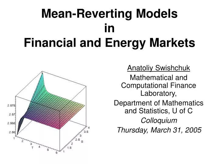
Mean-Reverting Models in Financial and Energy Markets Anatoliy Swishchuk Mathematical and Computational Finance Laboratory, Department of Mathematics and Statistics, U of C Colloquium Thursday, March 31, 2005
Outline • Mean-Reverting Models (MRM): Deterministic vs. Stochastic • MRM in Finance: Variances (Not Asset Prices) • MRM in Energy Markets: Asset Prices • Some Results: Swaps, Swaps with Delay, Option Pricing Formula (one-factor models) • Drawback of One-Factor Models • Future Work
Mean-Reversion Effect • Violin (or Guitar) String Analogy: if we pluck the violin (or guitar) string, the string will revert to its place of equilibrium • To measure how quickly this reversion back to the equilibrium location would happen we had to pluck the string • Similarly, the only way to measure mean reversion is when the variances of asset prices in financial markets and asset prices in energy markets get plucked away from their non-event levels and we observe them go back to more or less the levels they started from
Meaning of Mean-Reverting Parameter • The greater the mean-reverting parameter value, a, the greater is the pull back to the equilibrium level • For a daily variable change, the change in time, dt, in annualized terms is given by 1/365 • If a=365, the mean reversion would act so quickly as to bring the variable back to its equilibrium within a single day • The value of 365/a gives us an idea of how quickly the variable takes to get back to the equilibrium-in days
Mean-Reverting Models in Financial Markets • Stock (asset) Prices follow geometric Brownian motion • The Variance of Stock Price follows Mean-Reverting Models
Mean-Reverting Models in Energy Markets • Asset Prices follow Mean-Reverting Stochastic Processes
Heston Model for Stock Price and Variance Model for Stock Price (geometric Brownian motion): or deterministic interest rate, follows Cox-Ingersoll-Ross (CIR) process
Standard Brownian Motion andGeometric Brownian Motion Standard Brownian motion Geometric Brownian motion
Heston Model: Variance follows mean-reverting (CIR) process or
Cox-Ingersoll-Ross (CIR) Model for Stochastic Variance (Volatility) The model is a mean-reverting process, which pushes away from zero to keep it positive. The drift term is a restoring force which always points towards the current mean value .
Stock (a security representing partial ownership of a company) Bonds (bank accounts) Option (right but not obligation to do something in the future) Forward contract (an agreement to buy or sell something in a future date for a set price: obligation) Swaps-agreements between two counterparts to exchange cash flows in the future to a prearrange formula: obligation Swaps Security-a piece of paper representing a promise Basic Securities Derivative Securities
Volatility swaps are forward contracts on future realized stock volatility Variance swaps are forward contract on future realized stock variance Variance and Volatility Swaps Forward contract-an agreement to buy or sell something at a future date for a set price (forward price) Variance is a measure of the uncertainty of a stock price. Volatility (standard deviation) is the square root of the variance (the amount of “noise”, risk or variability in stock price) Variance=(Volatility)^2
Realized Continuous Variance and Volatility Realized (or Observed) Continuous Variance: Realized Continuous Volatility: where is a stock volatility, is expiration date or maturity.
Variance Swaps A Variance Swap is a forward contract on realized variance. Its payoff at expiration is equal to (Kvaris the delivery price for variance and N is the notional amount in $ per annualized variance point)
Volatility Swaps A Volatility Swap is a forward contract on realized volatility. Its payoff at expiration is equal to:
Example: Payoff for Volatility and Variance Swaps For Volatility Swap: a) volatility increased to 21%: Strike price Kvol =18% ; Realized Volatility=21%; N=$50,000/(volatility point). Payment(HF to D)=$50,000(21%-18%)=$150,000. b) volatility decreased to 12%: Payment(D to HF)=$50,000(18%-12%)=$300,000. For Variance Swap: Kvar = (18%)^2;N =$50,000/(one volatility point)^2.
Valuing of Variance Swap forStochastic Volatility Value of Variance Swap (present value): where E is an expectation (or mean value), r is interest rate. To calculate variance swap we need only E{V}, where and
Valuing of Volatility Swap for Stochastic Volatility Value of volatility swap: We use second order Taylor expansion for square root function. To calculate volatility swap we need not only E{V} (as inthe case of variance swap), but also Var{V}.
Calculation of Var[V] (continuation) After calculations: Finally we obtain:
Numerical Example: S&P60 Canada Index • We apply the obtained analytical solutions to price a swap on the volatility of the S&P60 Canada Index for five years (January 1997-February 2002) • These data were kindly presented to author by Raymond Theoret (University of Quebec, Montreal, Quebec,Canada) and Pierre Rostan (Bank of Montreal, Montreal, Quebec,Canada)
Logarithmic Returns Logarithmic returns are used in practice to define discrete sampled variance and volatility Logarithmic Returns: where
Statistics on Log-Returns of S&P60 Canada Index for 5 years (1997-2002)
Realized Continuous Variance forStochastic Volatility with Delay Stock Price Initial Data deterministic function
Equation for Stochastic Variance with Delay (Continuous-Time GARCH Model) Our (Kazmerchuk, Swishchuk, Wu (2002) “The Option Pricing Formula for Security Markets with Delayed Response”) first attempt was: This is a continuous-time analogue of its discrete-time GARCH(1,1) model J.-C. Duan remarked that it is important to incorporate the expectation of log-return into the model
Stochastic Volatility with Delay Main Features of this Model • Continuous-time analogue of GARCH(1,1) • Mean-reversion • Does not contain another Wiener process • Complete market • Incorporates theexpectation of log-return
Valuing of Variance Swap forStochastic Volatility with Delay Value of Variance Swap (present value): where E is an expectation (or mean value), r is interest rate. To calculate variance swap we need only E{V}, where and
Deterministic Equation for Expectation of Variance with Delay There is no explicit solution for this equation besides stationary solution.
Valuing of Variance Swap with Delay in General Case We need to find EP*[Var(S)]:
Dependence of Variance Swap with Delay on Maturity (S&P60 Canada Index)
Explicit Option Pricing Formula for European Call Option under Physical Measure