Download
1 / 34
340 likes | 587 Views
Chapter 10 Index models for Portfolio Selection. By Cheng Few Lee Joseph Finnerty John Lee Alice C Lee Donald Wort. Chapter Outline. 10.1 THE SINGLE-INDEX MODEL 10.1.1Deriving the Single-Index Model 10.1.1.1 Expected Return of a Portfolio 10.1.1.2 Variance of a Portfolio

E N D
Chapter 10Index models for Portfolio Selection By Cheng Few Lee Joseph Finnerty John Lee Alice C Lee Donald Wort
Chapter Outline 10.1 THE SINGLE-INDEX MODEL 10.1.1Deriving the Single-Index Model 10.1.1.1 Expected Return of a Portfolio 10.1.1.2 Variance of a Portfolio 10.1.2 Portfolio Analysis and the Single-Index Model 10.1.3 The Market Model and Beta 10.2 MULTIPLE INDEXES AND THE MIM 10.3 SUMMARY
10.1 The Single-Index Model (10.1) The essential difference between the single- and multiple-index models is the assumption that the single-index model explains the return of a security or a portfolio with only the market. The multiple-index model describes portfolio returns through the use of more than one index. Suggested by Markowitz (1959), the single-index model was fully developed by Sharpe (1970), who assumed that the covariances could be overlooked. The return of an individual security was tied to two factors-a random effect and the performance of some underlying market index. Notationally: where: ai and bi = regression parameters for the ith firm; = the return of some underlying market index at time t; = the return on security I at time t; and = the random effect for the ith security at time t.
Equation (10.1) makes several assumptions about the random effect term, full details are in text book page 354. • The expected value of the return on security i is equal to the sum of the intercept, the adjusted return on the index, and some random effect. • This can be expressed: • Because are constants, and is equal to zero: Where is equal to the mean of the returns on the market index. (10.2) (10.3)
(10.4) (10.5) If the mean of the returns on security i equals then the variance of security i is equal to the expected value of squared deviations from . This translates to By the third assumption, the covariance of the random effect and the deviation of the index return from its mean are zero; also, the expected value of the squared errors is equal to the variance of the random effect. Thus:
(10.6) It is suggested that because variations in the returns of two different securities are not interrelated but only connected to the market index, the covariance between the two securities can be derived from the twice-adjusted variance of the market index (once by the b coefficient of the first security with the market and again by the b coefficient of the second security with the market). The investigation starts with a statement about the covariance of the two securities:
(10.7) • Since according to the third and fourth assumptions the last three terms of the last summation are equal to zero: • For a portfolio with a hundred securities, this translates to 5,050 calculations. • With the Sharpe single-index model, only 100 estimates are needed for the various security-regression coefficients and only one variance calculation, the variance of the returns on the market. • In addition, 100 estimates of the unsystematic risk are also needed for the single-index model. • Hence, the single-index model has dramatically reduced the input information needed.
10.1.1 Deriving the Single-Index Model 10.1.1.1 Expected Return of a Portfolio • So far only the Sharpe single-index model has been utilized to study the return of a single security ias determined by its relation to the returns on a market index. • Now consider the return of a portfolio of n securities. • The return of a portfolio of n securities is the weighted summation of the individual returns of the component securities. • Notationally: where Rpt is the rate of return for a portfolio in period t and Xiis the weight associated with the ith security.
(10.8a) (10.8b) Thus, This equation indicates that the return of a portfolio may be decomposed into the summation of the weighted returns peculiar to the individual securities and the summation of the weighted adjusted return on the market index. Thus the portfolio may be viewed as a combination of n basic securities and a weighted adjusted return from an investment in the market index.
10.1.1.2 Variance of a Portfolio • To derive the variance of the portfolio , consider first that the mean return of the portfolio is equal to the expected value of the return on the portfolio. • Because the weighted sum of the coefficients is equal to the coefficient of the portfolio ,similarly . Hence, the last equation reduces to • In Equation (10.10) the last term, the weighted sum of the random effect variances, approaches zero as n increases. (10.9) (10.10)
Sample Problem 10.1 Solution: Substituting the related information into Equation (10.10): Therefore, bp = 1.414 Given the following information, what should the of the portfolio (bp) be?
Equation (10.8b) implies that the portfolio can be viewed as an investment in n basic securities and a weighted adjusted return in the market, or • The return on the market can be decomposed as a combination of the expected return plus some random effect. • When this random effect is positive, the atmosphere is bullish and when it is negative, the atmosphere is bearish. • Notationally: • This bit of algebraic maneuvering enables the weighted adjusted investment in the market to be viewed as an investment in an artificial security, the (n+1)th of an n-security portfolio. (10.11)
(10.12) (10.13) The weight for this (n+l)th security is the sum of the n weights multiplied by their respective related coefficients to the market index. Thus: The reason for this divergence in notation resulting in the definition of the (n+l)th security’s return and weight is that Equation (10.8) can be simplified to yield a working model for portfolio analysis. Substituting the last results for and into Equation (10.8B) yields:
(10.14) (10.15) Because the expected value of the random-effect terms is zero, the summation that results after the application of the expectations operator can be expressed as This yields a formula for the return of a portfolio that is easily applied to portfolio analysis. Before proceeding, however, it is necessary to simplify the variance formula so that it may be used as well. Remembering that the variance of the portfolio is the expected value of the squared deviations from the expected market return, the last results concerning and may be applied: This result follows from the assumption that the covariances are equal to zero.
Sample Problem 10.2 GivenRIt, Rit and as indicated in the Table 10.1 shown below and the fact that , using the relationship find the values for , and . Table 10.1 Single Index Model
Solution: • Substitute the values , n = 4 into the regression line • and solve for . • The column in Table 10.1 is filled by simply multiplying by the column. • The ‘s are the amounts such that is an equality, so is satisfied. • From the last column of the table we know that • Therefore • In this section, the expected return and the variance of a portfolio in terms of the single-index model has been derived.
10.1.2 Portfolio Analysis and the Single-Index Model (10.16a) (10.16b) • The first constraint is equivalent to requiring that the sum of the weights of the component securities is equal to one. • The second constraint requires that the weight of the market index within the portfolio returns is equal to the summation of the weighted adjustment factors of the component securities. • Combining the above two objective functions with the two constraints yields a Lagrangian function: The maximization procedure maximizes a linear combination of the following two equations:
Figure 10.1 Level of Risk Aversion and Investors’ Investment Attitude When low values are exhibited, risk aversion is pronounced; when high values are in evidence, substantial risk taking is allowed. This notion of the level of risk aversion is best pictured in Figure 10.1. In Figure 10.1, A represents an investor’s objective function to minimize the risk only-therefore, the aggressiveness to return is zero. C represents an investor’s objective function to maximize returns only-therefore, the aggressiveness to return is infinite. At B an investor’s attitude toward return and risk is between A and C.
Figure 10.2 Level of Risk Aversion and Object Function Figure 10.2 provides further illustration of the approach being utilized. What is depicted is the variation of the objective function P as the parameter denoting risk is varied. Points A and C are as discussed for Figure 10.1. Lines BD and B’D’represent the objective function when the risk-aversion parameter is equal to one. Note that BD instead of represents the maximization of the objective function. In sum, different values of generate different optimal objective functions.
(10.17) (10.18) Now consider the three-security portfolio. In this framework, the preceding objective function expands to: To proceed with the Lagrangian maximization it is necessary to notice that the above equation has six unknowns — the four weights and the two Lagrangian coefficients. All other values are expected to be known or estimated. To maximize, the partial derivative of the objective function is taken with respect to each of the six variables:
Equation (10.18) is a set of six equations in six unknowns when set equal to zero. These six equations can be rewritten in matrix format: • Equation (10.19A) has related the individual securities to the index and has discarded the use of numerous covariance terms. The majority of the elements of the matrix indicated in the first matrix of Equation (10.19A) are zero. • The majority of the elements of the matrix indicated in the first matrix of Equation (l0.19a) are zero. For three securities case, the inputs needed for Equation (10.19a) are three alphas, three betas, and three residual variances for individual securities. (10.19a)
As in Chapter 8, to solve for the x column vector of variables the P matrix is inverted and each side of the equation is premultiplied by . • This yields the x column vector of variables on the left-hand side and multiplied by k, the solution column vector, on the right-hand side. • where I is the identity matrix. • In order to estimate a single-index type of optimal portfolio the estimates of a market model are needed; a discussion of the market model and beta estimates is therefore needed as well. (10.19b)
Sample Problem 10.3 • During the discussion of the single-index model, a method was presented for determining optimal portfolio weights given different levels of risk aversion. • In this section a three-security portfolio is examined in which the returns of the securities are related to a market index. • The securities and the index have the following observed parameter estimates taken from actual monthly returns during the period from April 2000 to April 2010 (see Table 10-2). • The table includes the calculation of the beta estimate for each security. • Check these figures, remembering that beta is equal to the covariance of security iwith the market divided by the variance of the market returns. Table 10.2 Single Index Model: Three Securities Case
A matrix can be developed by utilizing the set of data in the first table of this problem and a of 1.0 (denoting moderate risk aversion): When the P matrix is invented and premultiplies each side of the equation:
This solution vector shows that investment should be divided 170.92% in JNJ, −68.21% in IBM, and −2.71% in BA. • Additionally, the weight of is the sum of the weighted adjustments as indicated in Equation (10.16b). • The return on this portfolio is the weighted sum of the individual returns: • The variance of the portfolio is the sum of the weighted variance and covariance terms:
Taking the covariance expressions: • A portfolio has been developed that is efficient within the realm of this model. • By varying the utility factor from risk averse to more aggressive risk posture we can develop an efficient frontier under the Sharpe single-index model. • For a fuller graph, the analyst would continue the calculations with ever higher values of stretching the efficient frontier.
10.1.3 The Market Model and Beta • Equation (10.1) defines the market model: • From this market model ai, bi, Var(ei), andVar(RIt) can be estimated: all are required for the single-index type of optimal portfolio. • So far the regression coefficient has been referred to as bi when, in fact, it is a risk relationship of a security with the market. • Quantified as the covariance of security iwith the market index divided by the variance of the return of the market, beta is a relational coefficient of the returns of security ias they vary with the returns of the market. • Notationally: • Of course, due to the continuous nature of security returns, the result of the above calculation is an estimate and therefore subject to error. • This error can be quantified by the use of standard error estimates, which provide the ability to make interval estimations for future predictions. (10.1) (10.20)
Because of the linkage between security returns and the firm’s underlying fundamental nature, beta estimates will vary over time. • It is the job of the security analyst to decide how to modify not only the beta estimate but also the period of time from which the sample of returns is to be drawn. • Some popular security-evaluation techniques use a tiered growth model to correspond to the product life-cycle theory. • Within the scope of this theory, beta estimates for the relation of that security to the market will vary with respect to the time period chosen for the sample of returns. • It is obvious that the returns generated by a firm in its infancy have very little correlation with returns during the growth or maturity phase. • It is up to the analyst to judge which phase a company may be in and to adjust the beta estimates accordingly. • This section has briefly looked over some of the available adjustment processes for beta estimation.
10.2 Multiple Indexes and the MIM • The multi-index model (MIM) pursues the same problem as beta adjustment, but approaches the problem from a different angle. • The MIM tackles the problem of relation of a security not only to the market by including a market index but also to other indexes that quantify other movements. • The covariance of a security’s return with other market influences can be added directly to the index model by quantifying the effects through the use of additional indexes. • If the single-index model were expanded to take into account interest rates, factory orders, and several industry-related indexes, the model would change to: • In this depiction of the MIM, is the actual level of index j, while is the actual responsiveness of security i to index j. (10.21)
(10.22) Assume there is a hypothetical model that deals with two indexes: Suppose the indexes are the market index and an index of wholesale prices. If these two indexes are correlated, the correlation may be removed from either index. To remove the relation between and , the coefficients of the following equation can be derived by regression analysis:
By the assumptions of regression analysis, is uncorrelated with. Therefore: which is an index of the performance of the sector index without the effect of I1(the market removed). Defining: an index is obtained that is uncorrelated with the market. By solving for and substituting into Equation (10.22): Rearranging • If the first set of terms in the brackets are defined asand the second set of terms are defined as , = , = and ci=ei , the equation can be expressed: (10.23) • in which are totally uncorrelated: the goal has been achieved. • As will be seen later, these simplifying calculations will make the job of determining variance and covariance much simpler.
The expected return can be expressed: (10.24) Variance can be expressed:
But by assumption: and Therefore, (10.25) Covariance between security iand security j can be expressed: (10.26)
10.3 SUMMARY • This chapter has discussed the essentials of single- and multiple-index models. • The theoretical underpinnings of the theories have been explored and numerical examples have been provided. • An efficient boundary has been derived under the guidelines of the model and the quantitative analysis of the related parameters has been studied. • It has been shown that both single-index and multi-index models can be used to simplify the Markowitz model for portfolio section; remember, however, that the multi-index model is much more complicated than the single-index model.