Download
1 / 45
450 likes | 518 Views
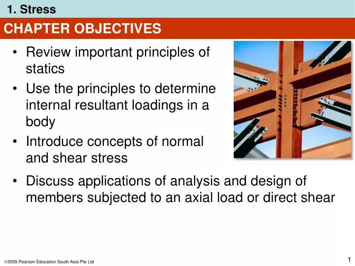
CHAPTER OBJECTIVES. Review important principles of statics Use the principles to determine internal resultant loadings in a body Introduce concepts of normal and shear stress. Discuss applications of analysis and design of members subjected to an axial load or direct shear. CHAPTER OUTLINE.

E N D
CHAPTER OBJECTIVES • Review important principles of statics • Use the principles to determine internal resultant loadings in a body • Introduce concepts of normal and shear stress Discuss applications of analysis and design of members subjected to an axial load or direct shear
CHAPTER OUTLINE • Introduction • Equilibrium of a deformable body • Stress • Average normal stress in an axially loaded bar • Average shear stress • Allowable stress • Design of simple connections
1.1 INTRODUCTION Mechanics of materials • A branch of mechanics • It studies the relationship of • External loads applied to a deformable body, and • The intensity of internal forces acting within the body • Are used to compute deformations of a body • Study body’s stability when external forces are applied to it
1.1 INTRODUCTION Historical development • Beginning of 17th century (Galileo) • Early 18th century (Saint-Venant, Poisson, Lamé and Navier) • In recent times, with advanced mathematical and computer techniques, more complex problems can be solved
1.2 EQUILIBRIUM OF A DEFORMABLE BODY External loads • Surface forces • Area of contact • Concentrated force • Linear distributed force • Centroid C (or geometric center) • Body force (e.g., weight)
1.2 EQUILIBRIUM OF A DEFORMABLE BODY Support reactions • for 2D problems
∑F = 0 ∑MO = 0 1.2 EQUILIBRIUM OF A DEFORMABLE BODY Equations of equilibrium • For equilibrium • balance of forces • balance of moments • Draw a free-body diagram to account for all forces acting on the body • Apply the two equations to achieve equilibrium state
1.2 EQUILIBRIUM OF A DEFORMABLE BODY Internal resultant loadings • Define resultant force (FR) and moment (MRo) in 3D: • Normal force, N • Shear force, V • Torsional moment or torque, T • Bending moment, M
1.2 EQUILIBRIUM OF A DEFORMABLE BODY Internal resultant loadings • For coplanar loadings: • Normal force, N • Shear force, V • Bending moment, M
1.2 EQUILIBRIUM OF A DEFORMABLE BODY Internal resultant loadings • For coplanar loadings: • Apply ∑ Fx = 0 to solve forN • Apply ∑ Fy = 0 to solve for V • Apply ∑ MO = 0 to solve for M
1.2 EQUILIBRIUM OF A DEFORMABLE BODY Procedure for analysis • Method of sections • Choose segment to analyze • Determine Support Reactions • Draw free-body diagram for whole body • Apply equations of equilibrium
1.2 EQUILIBRIUM OF A DEFORMABLE BODY Procedure for analysis • Free-body diagram • Keep all external loadings in exact locations before “sectioning” • Indicate unknown resultants, N, V, M, and T at the section, normally at centroid C of sectioned area • Coplanar system of forces only include N, V, and M • Establish x, y, z coordinate axes with origin at centroid
1.2 EQUILIBRIUM OF A DEFORMABLE BODY Procedure for analysis • Equations of equilibrium • Sum moments at section, about each coordinate axes where resultants act • This will eliminate unknown forces N and V, with direct solution for M (and T) • Resultant force with negative value implies that assumed direction is opposite to that shown on free-body diagram
EXAMPLE 1.1 Determine resultant loadings acting on cross section at C of beam.
EXAMPLE 1.1 (SOLN) Support reactions • Consider segment CB Free-body diagram: • Keep distributed loading exactly where it is on segment CBafter “cutting” the section. • Replace it with a single resultant force, F.
Intensity (w) of loading at C (by proportion) w/6 m = (270 N/m)/9 m w = 180 N/m F = ½ (180 N/m)(6 m) = 540 N F acts 1/3(6 m) = 2 m from C. EXAMPLE 1.1 (SOLN) Free-body diagram:
∑ Fx= 0; − Nc = 0 Nc = 0 ∑ Fy= 0; Vc− 540 N = 0 Vc = 540 N + + ∑ Mc = 0; −Mc− 504 N (2 m) = 0 Mc = −1080 N·m + EXAMPLE 1.1 (SOLN) Equilibrium equations:
EXAMPLE 1.1 (SOLN) Equilibrium equations: Negative sign of Mc means it acts in the opposite direction to that shown below
EXAMPLE 1.5 Mass of pipe = 2 kg/m, subjected to vertical force of 50 N and couple moment of 70 N·m at end A. It is fixed to the wall at C. Determine resultant internal loadings acting on cross section at B of pipe.
EXAMPLE 1.5 (SOLN) Support reactions: • Consider segment AB, which does not involve support reactions at C. Free-body diagram: • Need to find weight of each segment.
EXAMPLE 1.5 (SOLN) WBD = (2 kg/m)(0.5 m)(9.81 N/kg) = 9.81 N WAD = (2 kg/m)(1.25 m)(9.81 N/kg) = 24.525 N
(FB)x = 0 ∑Fx = 0; ∑Fy = 0; (FB)y = 0 ∑Fz = 0; (FB)z− 9.81 N − 24.525 N − 50 N = 0 (FB)z = 84.3 N EXAMPLE 1.5 (SOLN) Equilibrium equations:
EXAMPLE 1.5 (SOLN) Equilibrium equations: ∑ (MB)x = 0; (Mc)x + 70 N·m − 50 N (0.5 m) − 24.525 N (0.5 m) − 9.81 N (0.25m) = 0 (MB)x= − 30.3 N·m ∑ (MB)y = 0; (Mc)y + 24.525 N (0.625·m) + 50 N (1.25 m) = 0 (MB)y= − 77.8 N·m (Mc)z = 0 ∑(MB)z = 0;
NB = (FB)y = 0 VB = √ (0)2 + (84.3)2 = 84.3 N TB = (MB)y = 77.8 N·m MB = √ (30.3)2 + (0)2 = 30.3 N·m EXAMPLE 1.5 (SOLN) Equilibrium equations: The direction of each moment is determined using the right-hand rule: positive moments (thumb) directed along positive coordinate axis
1.3 STRESS Concept of stress • To obtain distribution of force acting over a sectioned area • Assumptions of material: • It is continuous (uniform distribution of matter) • It is cohesive (all portions are connected together)
1.3 STRESS Concept of stress • Consider ΔA in figure below • Small finite force, ΔF acts on ΔA • As ΔA → 0, ΔF → 0 • But stress (ΔF / ΔA) → finite limit (∞)
ΔFz ΔA lim ΔA →0 σz = 1.3 STRESS Normal stress • Intensity of force, or force per unit area, acting normal to ΔA • Symbol used for normal stress, is σ (sigma) Tensile stress: normal force “pulls” or “stretches” the area element ΔA Compressive stress: normal force “pushes” or “compresses” area element ΔA
ΔFx ΔA lim ΔA →0 τzx = ΔFy ΔA lim ΔA →0 τzy = 1.3 STRESS Shear stress • Intensity of force, or force per unit area, acting tangent to ΔA • Symbol used for normal stress is τ (tau)
1.3 STRESS General state of stress • Figure shows the state of stress acting around a chosen point in a body Units (SI system) • Newtons per square meter (N/m2) or a pascal (1 Pa = 1 N/m2) • kPa = 103 N/m2 (kilo-pascal) • MPa = 106 N/m2 (mega-pascal) • GPa = 109 N/m2 (giga-pascal)
1.4 AVERAGE NORMAL STRESS IN AXIALLY LOADED BAR Examples of axially loaded bar • Usually long and slender structural members • Truss members, hangers, bolts • Prismatic means all the cross sections are the same
1.4 AVERAGE NORMAL STRESS IN AXIALLY LOADED BAR Assumptions • Uniform deformation: Bar remains straight before and after load is applied, and cross section remains flat or plane during deformation • In order for uniform deformation, force P be applied along centroidal axis of cross section
FRz = ∑ Fxz ∫ dF = ∫Aσ dA P = σA P A σ = + 1.4 AVERAGE NORMAL STRESS IN AXIALLY LOADED BAR Average normal stress distribution σ= average normal stress at any point on cross sectional area P = internal resultant normal force A = x-sectional area of the bar
∑ Fz = 0 σ (ΔA) − σ’ (ΔA) = 0 σ = σ’ 1.4 AVERAGE NORMAL STRESS IN AXIALLY LOADED BAR Equilibrium • Consider vertical equilibrium of the element Above analysis applies to members subjected to tension or compression.
1.4 AVERAGE NORMAL STRESS IN AXIALLY LOADED BAR Maximum average normal stress • For problems where internal force P and x-sectional A were constant along the longitudinal axis of the bar, normal stress σ= P/A is also constant • If the bar is subjected to several external loads along its axis, change in x-sectional area may occur • Thus, it is important to find the maximum average normal stress • To determine that, we need to find the location where ratio P/A is a maximum
1.4 AVERAGE NORMAL STRESS IN AXIALLY LOADED BAR Maximum average normal stress • Draw an axial or normal force diagram (plot of P vs. its position x along bar’s length) • Sign convention: • P is positive (+) if it causes tension in the member • P is negative (−) if it causes compression • Identify the maximum average normal stress from the plot
1.4 AVERAGE NORMAL STRESS IN AXIALLY LOADED BAR Procedure for analysis Average normal stress • Use equation of σ = P/A for x-sectional area of a member when section subjected to internal resultant force P
1.4 AVERAGE NORMAL STRESS IN AXIALLY LOADED BAR Procedure for analysis Axially loaded members • Internal Loading: • Section member perpendicular to its longitudinal axis at pt where normal stress is to be determined • Draw free-body diagram • Use equation of force equilibrium to obtain internal axial force P at the section
1.4 AVERAGE NORMAL STRESS IN AXIALLY LOADED BAR Procedure for Analysis Axially loaded members • Average Normal Stress: • Determine member’s x-sectional area at the section • Compute average normal stress σ = P/A
EXAMPLE 1.6 Bar width = 35 mm, thickness = 10 mm Determine max. average normal stress in bar when subjected to loading shown.
EXAMPLE 1.6 (SOLN) Internal loading Normal force diagram By inspection, largest loading area is BC, where PBC = 30 kN
PBC A 30(103) N (0.035 m)(0.010 m) = 85.7 MPa σBC = = EXAMPLE 1.6 (SOLN) Average normal stress
EXAMPLE 1.8 Specific weight γst= 80 kN/m3 Determine average compressive stress acting at points A and B.
EXAMPLE 1.8 (SOLN) Internal loading Based on free-body diagram, weight of segment AB determined from Wst = γstVst
P− Wst = 0 P− (80 kN/m3)(0.8 m)(0.2 m)2 = 0 P = 8.042 kN ∑Fz = 0; + EXAMPLE 1.8 (SOLN) Average normal stress
8.042 kN (0.2 m)2 P A = σ = σ = 64.0 kN/m2 EXAMPLE 1.8 (SOLN) Average compressive stress Cross-sectional area at section: A = (0.2)m2