Download
1 / 41
410 likes | 656 Views
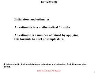
ESTIMATORS. Estimators and estimates: An estimator is a mathematical formula. An estimate is a number obtained by applying this formula to a set of sample data. It is important to distinguish between estimators and estimates. Definitions are given above. 1. ESTIMATORS.

E N D
ESTIMATORS Estimators and estimates: An estimator is a mathematical formula. An estimate is a number obtained by applying this formula to a set of sample data. It is important to distinguish between estimators and estimates. Definitions are given above. EMU, ECON 503, M. Balcılar 1
ESTIMATORS Population characteristic Estimator Mean: mX A common example of an estimator is the sample mean, which is the usual estimator of the population mean. EMU, ECON 503, M. Balcılar 4
ESTIMATORS Population characteristic Estimator Mean: mX Here it is defined for a random variable X and a sample of n observations. EMU, ECON 503, M. Balcılar 4
ESTIMATORS Population characteristic Estimator Mean: mX Population variance: Another common estimator is s2, defined above. It is used to estimate the population variance, sX2. EMU, ECON 503, M. Balcılar 4
ESTIMATORS Estimators are random variables An estimator is a special kind of random variable. We will demonstrate this in the case of the sample mean. EMU, ECON 503, M. Balcılar 8
ESTIMATORS Estimators are random variables We saw in the previous sequence that each observation on X can be decomposed into a fixed component and a random component. EMU, ECON 503, M. Balcılar 8
ESTIMATORS Estimators are random variables So the sample mean is the average of n fixed components and n random components. EMU, ECON 503, M. Balcılar 8
ESTIMATORS Estimators are random variables It thus has a fixed component mXand a random component u, the average of the random components in the observations in the sample. EMU, ECON 503, M. Balcılar 8
ESTIMATORS probability density function of X probability density function of X mX X mX X The graph compares the probability density functions of X and X. As we have seen, they have the same fixed component. However the distribution of the sample mean is more concentrated. EMU, ECON 503, M. Balcılar 10
ESTIMATORS probability density function of X probability density function of X mX X mX X Its random component tends to be smaller than that of X because it is the average of the random components in all the observations, and these tend to cancel each other out. EMU, ECON 503, M. Balcılar 10
UNBIASEDNESS AND EFFICIENCY Unbiasedness of X: Suppose that you wish to estimate the population mean mX of a random variable X given a sample of observations. We will demonstrate that the sample mean is an unbiased estimator, but not the only one. EMU, ECON 503, M. Balcılar 1
UNBIASEDNESS AND EFFICIENCY Unbiasedness of X: We use the second expected value rule to take the (1/n) factor out of the expectation expression. EMU, ECON 503, M. Balcılar 2
UNBIASEDNESS AND EFFICIENCY Unbiasedness of X: Next we use the first expected value rule to break up the expression into the sum of the expectations of the observations. EMU, ECON 503, M. Balcılar 3
UNBIASEDNESS AND EFFICIENCY Unbiasedness of X: Each expectation is equal to mX, and hence the expected value of the sample mean is mX. EMU, ECON 503, M. Balcılar 4
UNBIASEDNESS AND EFFICIENCY probability density function estimator B estimator A mX How do we choose among them? The answer is to use the most efficient estimator, the one with the smallest population variance, because it will tend to be the most accurate. EMU, ECON 503, M. Balcılar 12
UNBIASEDNESS AND EFFICIENCY probability density function estimator B estimator A mX In the diagram, A and B are both unbiased estimators but B is superior because it is more efficient. EMU, ECON 503, M. Balcılar 13
CONFLICTS BETWEEN UNBIASEDNESS AND MINIMUM VARIANCE probability density function estimator B estimator A q Suppose that you have alternative estimators of a population characteristic q, one unbiased, the other biased but with a smaller population variance. How do you choose between them? EMU, ECON 503, M. Balcılar 1
CONFLICTS BETWEEN UNBIASEDNESS AND MINIMUM VARIANCE loss error (negative) error (positive) One way is to define a loss function which reflects the cost to you of making errors, positive or negative, of different sizes. EMU, ECON 503, M. Balcılar 2
CONFLICTS BETWEEN UNBIASEDNESS AND MINIMUM VARIANCE probability density function estimator B q A widely-used loss function is the mean square error of the estimator, defined as the expected value of the square of the deviation of the estimator about the true value of the population characteristic. EMU, ECON 503, M. Balcılar 3
CONFLICTS BETWEEN UNBIASEDNESS AND MINIMUM VARIANCE probability density function estimator B bias q mZ The mean square error involves a trade-off between the population variance of the estimator and its bias. Suppose you have a biased estimator like estimator B above, with expected value mZ. EMU, ECON 503, M. Balcılar 4
CONFLICTS BETWEEN UNBIASEDNESS AND MINIMUM VARIANCE probability density function estimator B bias q mZ The mean square error can be shown to be equal to the sum of the population variance of the estimator and the square of the bias. EMU, ECON 503, M. Balcılar 5
CONFLICTS BETWEEN UNBIASEDNESS AND MINIMUM VARIANCE To demonstrate this, we start by subtracting and adding mZ . EMU, ECON 503, M. Balcılar 6
CONFLICTS BETWEEN UNBIASEDNESS AND MINIMUM VARIANCE We expand the quadratic using the rule (a + b)2 = a2 + b2 + 2ab, where a = Z - mZ and b = mZ - q. EMU, ECON 503, M. Balcılar 7
CONFLICTS BETWEEN UNBIASEDNESS AND MINIMUM VARIANCE We use the first expected value rule to break up the expectation into its three components. EMU, ECON 503, M. Balcılar 8
CONFLICTS BETWEEN UNBIASEDNESS AND MINIMUM VARIANCE The first term in the expression is by definition the population variance of Z. EMU, ECON 503, M. Balcılar 9
CONFLICTS BETWEEN UNBIASEDNESS AND MINIMUM VARIANCE (mZ - q) is a constant, so the second term is a constant. EMU, ECON 503, M. Balcılar 10
CONFLICTS BETWEEN UNBIASEDNESS AND MINIMUM VARIANCE In the third term, (mZ - q) may be brought out of the expectation, again because it is a constant, using the second expected value rule. EMU, ECON 503, M. Balcılar 11
CONFLICTS BETWEEN UNBIASEDNESS AND MINIMUM VARIANCE Now E(Z) is mZ, and E(-mZ) is -mZ. EMU, ECON 503, M. Balcılar 12
CONFLICTS BETWEEN UNBIASEDNESS AND MINIMUM VARIANCE Hence the third term is zero and the mean square error of Z is shown be the sum of the population variance of Z and the bias squared. EMU, ECON 503, M. Balcılar 13
CONFLICTS BETWEEN UNBIASEDNESS AND MINIMUM VARIANCE probability density function estimator B estimator A q In the case of the estimators shown, estimator B is probably a little better than estimator A according to the MSE criterion. EMU, ECON 503, M. Balcılar 14
EFFECT OF INCREASING THE SAMPLE SIZE ON THE DISTRIBUTION OF x probability density function of X n 1 50 0.08 0.06 0.04 0.02 n = 1 50 100 150 200 The sample mean is the usual estimator of a population mean, for reasons discussed in the previous sequence. In this sequence we will see how its properties are affected by the sample size. EMU, ECON 503, M. Balcılar 1
EFFECT OF INCREASING THE SAMPLE SIZE ON THE DISTRIBUTION OF x probability density function of X n 1 50 0.08 0.06 0.04 0.02 n = 1 50 100 150 200 Suppose that a random variable X has population mean 100 and standard deviation 50, as in the diagram. Suppose that we do not know the population mean and we are using the sample mean to estimate it. EMU, ECON 503, M. Balcılar 2
EFFECT OF INCREASING THE SAMPLE SIZE ON THE DISTRIBUTION OF x probability density function of X n 1 50 0.08 0.06 0.04 0.02 n = 1 50 100 150 200 The sample mean will have the same population mean as X, but its standard deviation will be 50/, where n is the number of observations in the sample. EMU, ECON 503, M. Balcılar 3
EFFECT OF INCREASING THE SAMPLE SIZE ON THE DISTRIBUTION OF x probability density function of X n 1 50 0.08 0.06 0.04 0.02 n = 1 50 100 150 200 The larger is the sample, the smaller will be the standard deviation of the sample mean. EMU, ECON 503, M. Balcılar 4
EFFECT OF INCREASING THE SAMPLE SIZE ON THE DISTRIBUTION OF x probability density function of X n 1 50 0.08 0.06 0.04 0.02 n = 1 50 100 150 200 If n is equal to 1, the sample consists of a single observation. X is the same as X and its standard deviation is 50. EMU, ECON 503, M. Balcılar 5
EFFECT OF INCREASING THE SAMPLE SIZE ON THE DISTRIBUTION OF x probability density function of X n 1 50 4 25 0.08 0.06 0.04 n = 4 0.02 50 100 150 200 We will see how the shape of the distribution changes as the sample size is increased. EMU, ECON 503, M. Balcılar 6
EFFECT OF INCREASING THE SAMPLE SIZE ON THE DISTRIBUTION OF x probability density function of X n 1 50 4 25 25 10 0.08 0.06 n = 25 0.04 0.02 50 100 150 200 The distribution becomes more concentrated about the population mean. EMU, ECON 503, M. Balcılar 7
EFFECT OF INCREASING THE SAMPLE SIZE ON THE DISTRIBUTION OF x probability density function of X n 1 50 4 25 25 10 100 5 n = 100 0.08 0.06 0.04 0.02 50 100 150 200 To see what happens for n greater than 100, we will have to change the vertical scale. EMU, ECON 503, M. Balcılar 8
EFFECT OF INCREASING THE SAMPLE SIZE ON THE DISTRIBUTION OF x probability density function of X n 1 50 4 25 25 10 100 5 0.8 0.6 0.4 n = 100 0.2 50 100 150 200 We have increased the vertical scale by a factor of 10. EMU, ECON 503, M. Balcılar 9
EFFECT OF INCREASING THE SAMPLE SIZE ON THE DISTRIBUTION OF x n = 1000 probability density function of X n 1 50 4 25 25 10 100 5 1000 1.6 0.8 0.6 0.4 0.2 50 100 150 200 The distribution continues to contract about the population mean. EMU, ECON 503, M. Balcılar 10
EFFECT OF INCREASING THE SAMPLE SIZE ON THE DISTRIBUTION OF x n = 5000 probability density function of X n 1 50 4 25 25 10 100 5 1000 1.6 5000 0.7 0.8 0.6 0.4 0.2 50 100 150 200 In the limit, the variance of the distribution tends to zero. The distribution collapses to a spike at the true value. The sample mean is therefore a consistent estimator of the population mean. EMU, ECON 503, M. Balcılar 11