Download
1 / 57
570 likes | 672 Views
Developing Marginal Cost-Based Rates. Kelly Eakin Senior Vice President Christensen Associates Energy Consulting APPA Business and Financial Conference Austin, TX September 25, 2007. Objectives of Presentation.

E N D
Developing MarginalCost-Based Rates Kelly Eakin Senior Vice President Christensen Associates Energy Consulting APPA Business and Financial Conference Austin, TX September 25, 2007
Objectives of Presentation • Provide a framework to evaluate social gains from marginal cost pricing and address the challenge of fixed cost recovery • Identify key determinants to marginal cost pricing gains • Look for ways to incorporate pricing efficiency principles into cost of service analysis
Business Objectives • Revenue Sufficiency • Maximizing stakeholder value
Outline • Economics Basics • The Regulatory Dilemma • Incorporating Marginal Cost Pricing Principles into Cost of Service Analysis • A Simple Stylized Example • Conclusions
Demand • Consumers are willing to pay for a good because it brings them some benefit or satisfaction • As more of a good is consumed, the additional or marginal benefit decreases (law of diminishing returns) • Consequently, the consumer’s willingness to pay for another unit of a good decreases as consumption increases • Law of Demand: Consumers will buy more of a good a lower prices, other things the same • Price Elasticity of Demand: • A measure of customer price responsiveness • εD = % change in quantity demanded ÷ % change in price
The Demand Curve Price P1 P2 D = marginal benefit Q1 Q2 QuantityDemanded
Costs • Costs reflect the “supply side” of a market • For goods to come to market, a supplier needs to expect at least to recover (variable) costs
Cost Measures (1) • Total Costs • Variable Cost – costs associated with the inputs that change as production levels change • Fixed Cost – costs that remain the same regardless of the production level, sometimes called “sunk costs” (e.g., capital costs) • Total Cost = Variable Cost + Fixed Cost or TC=VC+FC
Cost Measures (2) • Average Cost Concepts • Average Variable Cost (AVC) • Variable cost per unit of output: AVC=TVC/Q • Average Fixed Cost (AFC) • Fixed cost per unit of output: AFC/Q • AFC decreases as output increases (spreading out the overhead) • Average Total Cost (ATC) • Cost per unit of output: • ATC = TC/Q • ATC = AVC +AFC The utility industry term “average embedded cost” corresponds closely to the economic term average total cost
Cost Measures (3) • Marginal Cost (MC) • Marginal cost measures how cost changes as an additional unit of output is produced • MC = ∆TC/∆Q = ∆TVC/∆Q • Marginal cost is the supply schedule for a competitive profit-maximizing firm • A supply schedule is more ambiguous if there is a lack of competition or the firm is not a profit maximizer
Cost Measures (4) • Fixed Costs • Common cost—overhead costs that occurs regardless of product lines offered, production levels or customer classes served • Class-specific fixed cost—costs that do not vary with production levels but that are avoidable if a customer class is not served • Product-specific fixed cost—costs that do not vary with production levels but that are avoidable if a product line is not produced • Fixed cost recovery can introduce price distortion and resulting social value loss (called economic inefficiency)
Cost Measures (5) • Incremental Cost (ICi) • Incremental cost indicates the additional cost of adding a product line or serving another customer class • Subtle differences from marginal cost • Discrete change instead of incremental change • May involve some product/class specific fixed (but avoidable) costs • ICi = TC – TC without Qi = TC – TC(~ Qi) • Average Incremental Cost (AICi) • AICi = ICi/Qi • Important concept in investigating cross-subsidies
Cost Concepts (6) • Finally, pulling in some cost of service concepts • Attributable costs (or directly assigned costs) are those costs that can be assigned as “caused” by serving a customer class • Variable costs • Class-specific fixed costs • Product-specific fixed costs for products serving only one customer class • Non-attributable costs—those costs that occur regardless of whether a particular customer class is served • Common costs • Product-specific fixed costs for products serving all customer classes
Cross-Subsidization • Charging some more than attributable cost so that others pay less than their attributable cost • Different criteria for cross-subsidization • Price vs. Average Total Cost • Price vs. Average Variable Cost • Price vs. Marginal Cost • Price vs. Average Incremental Cost • Cross-subsidization involves • Inefficiency • Fairness issue
Cross-Subsidization • Pi < AICi • Revenue from class less than its incremental cost • Serving the class adds to the overhead contribution required from other classes • Other classes would pay less if this class were not served • The class is receiving a cross-subsidy from other classes • Pi = AICi • Revenue just covers incremental cost but class makes no contribution to overhead • No impact on other classes • No cross-subsidy • Pi > AICi • Revenue from class more than its incremental cost • the class makes a contribution to overhead • Other classes would pay more if this class were not served • No cross-subsidy
Economic Efficiency • Economic efficiency occurs when resources are used in a way that generates the greatest economic value • Price = Marginal Cost is the efficiency condition • P > MC too little produced; additional value would exceed additional cost • P < MC too much produced; additional cost of last unit more than offsets additional value • P=MC maximum net benefit; no way to reallocate resources to increase economic value
The Efficiency of Competition Firm Industry MC ATC S = MC P P D = MB q Q = nq
The Efficiency and Fairness of Competition • Efficiency • P = MC → economic output distributed to consumers in a manner that achieves the greatest economic value • MC = ATC → production is allocated among producers so that total production cost is minimized • Fairness • P = ATC → producers just break even covering their variable costs and earning a fair rate of return on capital investment; also called earning “normal profit” of “zero economic profit” • This condition is the result of no barriers to entry or exit The result of individuals pursuing self-interest, but the outcome is as if an “invisible hand” of a benevolent planner allocated the resources
Alas, competition and efficiency may not prevail • Industry might not be competitive • Barriers to entry • Large economies of scale • Firms might not be profit-maximizers • Public power has stakeholders rather than shareholders • Other non-profit organizations have objectives other than maximizing profit • Revenue adequacy still a requirement, but efficiency may not be a result
Natural Monopoly • Economies of scale exist if average cost decreases as a firm’s production increases • A natural monopoly has economies of scale over a large range of production relative to market demand • One firm can produce market output at a lower total cost than can two or more firms • Often have large overhead costs resulting from heavy capital investment (i.e., capital intensive industries) • Often involve basic needs such as water, electricity
Natural Monopoly $ ATC MC D Q
Rationale for Regulation • Promoting competition is inefficient in a natural monopoly situation • Instead rate regulation is the policy prescription • Called public utility regulation • Trying to achieve competitive-type (invisible hand) outcomes via regulation
The Not-So Invisible Hand of Regulation > “Cost-of-Service” Study Intervenor Discovery > Staff & Intervenors Prefile Testimony Staff & Intervenors Present Witnesses Company Presents Witnesses File Case Company Files Rebuttal Commission Order Commission Decision Submission of Briefs Cross Examination on Rebuttal > >
The Natural Monopoly Dilemma • A natural monopoly presents the regulator with a dilemma • Left unregulated, the monopolist could charge high prices resulting in inefficiency and a transfer of wealth from customers to the monopolist • Setting P=MC results in efficiency but insufficient revenues • Set P=ATC collects sufficient revenues but is inefficient • Issue becomes more complex with multiple products and customer classes
The Natural Monopoly Dilemma: P=MC is efficient but revenue inadequate $ ATC ATC Losses P MC D Q Q*
The Natural Monopoly Dilemma: P=ATC collects enough revenue but is inefficient $ Efficiency Loss ATC P = ATC MC D Q Q* Q
“Solutions” to the Pricing Dilemma • Simple markup pricing • Absolute markup: raise prices above marginal costs by the same amount to all classes • Proportional markup: raise prices above marginal costs by the same percent to all classes
“Solutions” to the Pricing Dilemma (2) • Differential markup pricing • Raise prices above marginal costs by different percentages to different classes • Ramsey Pricing raises prices differentially to minimize inefficiency • Price inverse to the elasticity of demand • Same pattern as what a monopolist would do, only to lesser magnitude
“Solutions” to the Pricing Dilemma (3) • Non-linear pricing • Collect some fixed costs via a non-volumetric charge (i.e., not per kWh or per kW) • If all fixed costs were collected non-volumetrically, then per unit charge could be set at marginal cost
Incorporating Marginal Cost Pricing Principles into Cost of Service Analysis Cost of Service Basics
Why investigate cost of service? • Improve understanding of the business • Help with rate design • Requirement for rate case
Basic Steps for a Traditional Cost of Service Study • Determine the Overall Revenue Requirement • Establish the customer classes • Attribute the attributable costs • Allocate the non-attributable costs • Set rates to achieve the revenue requirements
A Modified Approach: Marginal Cost-Based Cost of Service • Determine the Overall Revenue Requirement • Establish the customer classes • Attribute the attributable costs • Set preliminary prices at marginal costs • Conduct preliminary cross-subsidy analysis • Mark up prices to subsidized classes to eliminate cross-subsidies • Calculate revenue insufficiency • Mark up prices to all classes to achieve revenue requirement • Introduce revenue-neutral non-linear pricing to improve pricing efficiency
Challenges of the New Approach • Estimating the marginal costs • Costly to make numerous unbundled marginal cost estimates • Estimating marginal costs of ancillary services, transmission and distribution services is not trivial • Nevertheless, these marginal costs should be understood for business reasons beyond cost-of-service studies • Incorporating demand response into cost of service analysis • Essential for the pursuit of efficiency • Not a comparative disadvantage vis à vis traditional approach • Attributable costs may be a small fraction of total costs
Advantages of a Marginal Cost-BasedCost-of-Service Approach • Based on principles of economic efficiency • Knowledge of marginal cost has many useful business purposes separate of a cost-of-service study • Less arbitrary allocation of costs • May decrease the extent of cross-subsidization
Approaches to Allocating Common Cost • Method A: Divide total fixed costs by total usage • Ignores that some fixed costs are attributable • Ignores that marginal costs differ across classes • Allocation implicitly achieved by charging same price per kWh across all classes • Method B: Assign attributable fixed costs and allocate common cost on a per kWh basis • Method C: Assign attributable fixed costs and allocate common cost according to shares of attributable costs
Incorporating Demand Response • Assume the following price elasticities of demand (εD) εD Residential: -0.05 Commercial: -0.10 Industrial: -0.20 * Also assuming linear demand curve and using Method B prices and stipulated usage as the reference point
Recall the Efficiency Loss Triangle from Pricing Away from Marginal Cost $ Efficiency Loss ATC P = ATC MC D Q Q* Q
Economic Efficiency Analysis • The efficiency loss or deadweight loss (DWL) in each market can be approximated as DWL ≈ -½ εD (Q/P) (P-MC)2 • Pricing inefficiency requires both • Price differing from marginal cost • Existence of price responsiveness (εD≠0) • Determinants of the magnitude of value loss • Amount of fixed cost to be recovered • Size of the price distortion • Marginal cost • Price responsiveness