Download
1 / 44
470 likes | 828 Views
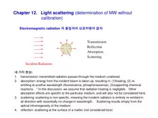
Chapter 12. Light scattering (determination of MW without calibration). Electromagnetic radiation 과 물질과의 상호작용의 결과. 네 가지 현상 : transmission: transmitted radiation passes through the medium unaltered.

E N D
Chapter 12. Light scattering (determination of MW without calibration) Electromagnetic radiation 과 물질과의 상호작용의 결과 • 네 가지 현상: • transmission: transmitted radiation passes through the medium unaltered. • absorption: energy from the incident beam is taken up, resulting in: (1)heating, (2) re-emitting at another wavelength (fluorescence, phosphorescence), (3)supporting chemical reactions. * In this discussion, we assume that radiation heating is negligible. Other absorption effects are specific to the particular medium, and will also not be considered here. • scattering: scattering is non-specific, meaning the incident radiation is entirely re-emitted in all direction with essentially no change in wavelength. Scattering results simply from the optical inhomogeneity of the medium. • reflection: scattering at the surface of a matter (not considered here)
Now we focus on the light scattering. • Application of Light Scattering for Analysis • Classical Light Scattering (CLS) or Static Light Scattering (SLS) • Dynamic Light Scattering (DLS, QELS, PCS) • CLS • 정의: Scattering center = small volumes of material that scatters light. 예: individual molecule in a gas. • Consequences of the interaction of the beam with the scattering center: depends, among other things, on the ratio of the size of the scattering center to the incident wavelength (λo). Our primary interest is the case where the radius of the scattering center, a, is much smaller than the wavelength of the incident light (a < 0.05λo, less than 5% of λo). This condition is satisfied by dissolved polymer coils of moderate molar mass radiated by VISIBLE light. When the oscillating electric field of the incident beam interacts with the scattering center, it induces a synchronous oscillating dipole, which re-emits the electromagnetic energy in all directions. Scattering under these circumstances is called Rayleigh scattering. The light which is not scattered is transmitted: , where Is and It are the intensity of the scattered and transmitted light, respectively.
Oscillating electric field of incident beam interacts with scattering center, induces a synchronous oscillating dipole, which re-emits electromagnetic energy in all directions. Rayleigh scattering에 의한 산란광의 세기는 측정 위치에 따라 변한다: (1+cos2θ)에 비례하고, scattering center와 observer사이의 거리(r)의 제곱에 반비례. • 1944, Debye • Rearrange: Constant, K λo = 입사광파장, dn/dc = refractive index increment no: 용매의 refractive index, π=삼투압, c=시료농도[g/mL]
Define “Rayleigh ratio” Rθ measured 얻고자 하는 정보 포함 Iθ is inversely proportional to λo. Shorter wavelength scatters more than longer wavelength Assume: system is dilute, the net signal at the point of observation is sum of all scattering intensities from individual scatterer - no multiple scattering (scattered light from one center strike another center causing re-scattering, etc.). • Two ways to access the light scattering information experimentally: • Turbidimeter (or spectrophotometer) • Light scattering
"Turbidity", τ = fraction of incident light which is scattered out = 1-(It/Io) • τ is obtained by integrating Iθ over all angles: Substitute: 1. Turbidimeter experiment (Transmitted light intensity, It is measured) Solution is dilute, so higher order concentration terms can be ignored.
Procedure: Measure τ at various conc. Plot Hc/T vs. c (straight line) Determine M from intercept, 2nd virial coeff., B from slope
2. Light Scattering experiment(measure Iθ at certain θ and r) 식6을 식4에 대입: *반경이 파장의 약 5% (λ/20) 이하인 경우에 국한됨 – “Rayleigh limit”
The slope of the plot can be either positive or negative. θ-condition에서 기울기=0.
(Hc)/τ vs. c 그래프의 절편 =1/M 이므로 <참고> For polydisperse sample, Turbidity (혹은 light scattering) is contributed by molecules of different MW. Define: τi= 분자량 Mi를 갖는 분자들에 의한 turbidity → 따라서 turbidity나 light scattering실험에서 얻는 분자량은 weight-average MW이다.
Rayleigh-Gans-Debye (RGD scattering) : when the scattering centers are larger than Rayleigh limit Different part of more extended domain (B) produce scattered light which interferes with that produced by other part (A) - constructive or destructive
a =반경 Q = scattering vector = (4π/λ)sin(θ/2)rg (10) 구형입자의 경우: Random coil 고분자의 경우, Distribution is symmetrical for small particles (<λ/20). For larger particles, intensity is reduced at all angles except zero. Contributions from two scattering centers can be summed to give the net scattering intensity. The result is a net reduction of the scattered intensity Pθ = "shape factor" or "form factor" Always Pθ < 1, function of size and shape of scattering volume. Now we start seeing the angle dependence of the scattered light !
p(θ) decreases with θ. • p(θ) decreases more for higher MW.
Effect of MW and Chain Conformation on Pθ, and on measured MW at 90o.
식(11)을 식(9)에 대입한 후 식(7’)에 대입: Random coil 고분자의 경우, Final Rayleigh equation for random coil polymer 두 가지 극한 상황: [Case 1]θ→0: Plot Kc/Rθ vs. c: y-절편=1/M, 기울기=2A2 [Case 2]c→0: Plot Kc/Rθ vs. sin2(θ/2): y-절편=1/M, 기울기= (16π2/3Mλ2) rg2 Three information!
빛산란 실험 방법 (1) 다양한 각도와 농도에서 Rθ측정. (2) Kc/Rθ vs. c, Kc/Rθ vs. sin2(θ /2) plot 작성. (3) θ =0와 c =0로 extrapolate. Kc/Rθ vs. sin2(θ /2) Kc/Rθ vs. c Zimm plot: 채워진 점: 실험 데이터. 빈 점: extrapolated points
(Kc/Rθ) vs. c Cases 1. Small polymers: 각도의존성 없음. (Horizontal line) Zimm plot for PMMA in butanone λo=546 nm, 25℃, no ~1.348, dn/dc = 0.112 cm3/g - 다섯 농도에서 측정한 데이터. - Mw 와 A2결정 가능 - 분자크기 측정 불가능. 2. Small polymers in θ-solvent: 각도 및 농도 의존성 없음. θ-solvent: A2=0가 되는 용매, 고분자-고분자, 고분자-용매분자간 상호작용의 에너지가 동일, 이상용액과 같이 행동. Zimm plot of poly(2-hydroxyethyl methacrylate) in isopropanol λo=436 nm, 25℃, no ~1.391, dn/dc = 0.125 cm3/g • Calculated values : Mw = 66,000 g/mol • A2 = 0 mol cm3/g2 • - Kc/Rθ at small angles fall mostly below the horizontal line plotted through the points from medium and large angles.
3. Larger polymers in good solvent: 각도 및 농도에 의존. Zimm plot of polystyrene in toluene λo=546 nm, 25℃, no ~1.498, dn/dc = 0.110 cm3/g - 분자량 약 2x10⁵이상의 경우, Kc/Rθ는 양의 기울기 (A2=양수)를 가진다. - Athermal Condition - No effect of temperature on polymer structure 4. Polymers in poor solvent: A2가 음수가 됨 (큰 음수는 될 수 없음. 더 이상 녹지 않기 때문) Zimm plot of polybutadiene in dioxane λo=546 nm, 25℃, no ~1.422, dn/dc = 0.110 cm3/g • - 각도의존성이 직선이 아님 (nonlinear). • - 이유: microgel, 먼지, aggregate과 같은 큰 입자 존재. • Curve-fitting에 주의를 요함. • 분자크기 측정의 정확도에 영향. • 분자가 커지면 good solvent에서도 • 직선성을 벗어날 수 있다.
Stand-alone vs. On-line MALS • <Stand-alone mode> • Stand-alone mode: LS instrument is used itself. • Zimm plot 을 이용 M, A2, Rθ를 결정 • <On-line mode> • LS instrument is used as a detector for a separator. • c=0 이라 가정. • 각 slice에 대해 Kc/Rθ vs. sin2(θ/2) 그래프를 이용, y-절편으로부터 분자량 (M), 초기기울기로부터 rg를 결정. y-절편=1/M, 초기기울기= (16π2/3Mλ2) rg2 • 각 slice가 monodisperse하다고 가정하고 평균분자량과 평균크기를 계산. 따라서 높은 분리도가 요구됨 (분리방법선택 및 분리최적화가 요구됨). • Average Molecular Weights • No-average: Mn=(Σci)/(Σ(ci/Mi)) • Wt-average: Mw=Σ(ciMi)/ Σ(ci) • Z-average: Mz= Σ(ciMi2)/Σ(ci/Mi) • Average Sizes (mean square radii) • No-average: <rg2>n= Σ[(ci/Mi)<rg2>i]/Σ(ci/Mi) • Wt-average: <rg2>w= Σ(ci<rg2>i)/Σci • Z-average: <rg2>z=Σ(ciMi<rg2>i)/Σ(ciMi)
(2) On-line mode: Assume c=0, Plot For each slice. Determine M from intercept (intercept = 1/M), rgfrom slope (slope = ) Light scattering instruments MALLS (Multi Angle Laser Light Scattering) : I is measured at 15 angles (1) Stand-alone mode: Measure scattered light at different angles for different concentrations Make a Zimm plot Determine M, B, Rg Assuming each slice is narrow distribution, Mw Mi Average M can be calculated. It is therefore very important to have a good resolution.
TALLS (Triple Angle): I is measured at 45o, 90o, and 135o • Not useful when the plot of deviates from linearity
Angular Dependence of Kc / R(시료= high molecular weight DNA)
Effect of Particles/Gels on Light Scattering Measurement Note the delicacy of extrapolation to zero angle from larger distances.
DALLS (Dual Angle): Iθ is measured at 15o and 90o • LALLS (Low Angle): Iθ is measured at one low angle (assume: = 0) • Static mode: measure LS at a few c Plot Kc/Rθ vs. c Determine M and B from intercept and slope. • On-line mode: determine Kc/Rθ for each slice ( calculate M). Considering each slice is narrow distribution, let Mw ( Mi, from which average MW's can be calculated (as learned in chapter 1). It is therefore again very important to have a good resolution. • RALLS (Right Angle) • Iθ is measured at 90o. • Simple design • Higher S/N ratio, Application is limited to cases where Pθ is close to 1 (e.g., less than 200K of linear random polymer) • RALLS combined with differential viscometer (commercially available from Viscotek, "TRISEC")
RG can be obtained using the Flory-Fox equation: Calculate P(θ=90). <TRISEC 이용방법> Assume Pθ = 1 and A2 = 0. Determine Mest. [η] is determined by differential viscometer, and M determined in step 2. Calculate new MW by Go to step 2. Repeat until Mest does not change.
<Light scattering experiment에필요한상수들> 에서K와B를제외한모든parameter는이미알고있다. 그런데 이므로다음세개의상수가필요. • n: 용매의refractive index • dn/dc : Specific refractive index increment • B: 2nd virial coefficient (Static mode에서는 B를 실험에 의해 결정할 수 있기 때문에 Static mode는 제외).
1. 용매의 Refractive Index • 거의 모든 용매에 대해 RI 값들이 알려져 있음. 자주쓰이는용매들 (R가감소하는순) • Except where otherwise noted, all measurements made at λ= 632.8 nm and T=23 oC. RI at 632.8 nm calculated by extrapolation from values measured at other wavelengths. • Extrapolation에관한reference: Johnson, B. L.; Smith, J. "Light Scattering from Polymer solutions" Huglin, M. B. ed., Academic press, New York, 1972, pp 27
2. Specific refractive Index, dn/dc • 문헌에서구할수있다(Polymer Handbook, Huglin, ed., Light Scattering from Polymer Solutions, Academic Press, 1972) • 문헌에서구할수없는경우실험에의해측정 • Conventional method • DRI를 이용 • 몇 가지 다른 농도에서 (n2-n1)을 측정 (recommended conc. = 2, 3, 4, 5 x 10⁻³ g/mL) → (n2-n1)/c2 vs. vs. c2를 plot → zero concentration으로 extrapolate → dn/dc는 intercept로 부 터 구한다.
For concentration ranges generally used, the refractive index difference, n2-n1, is a linear function of concentration. In other words, (n2-n1)/c2 is constant. 즉 (n2-n1)/c2 vs. c2그래프의 기울기=0. This means that (n2-n1) needs to be measured for only one or two different concentrations. If (n2-n1)/c2 shows no significant dependence on c, then dn/dc can be obtained by averaging (n2-n1)/c2 values
Ri = detector signal at the slice I kR = RI const ci = conc. (g/mL) of the slice i) → 시료를주입, dn/dc 계산: • SEC/RI를이용 • 이미 배운 바와 같이 먼저 dn/dc를아는표준시료를주입하여kR·을계산: • 문헌이나실험에의해구할수없는경우estimate을할수도있다. • extrapolate to desired wavelength: 혹은 2) polymer와 용매의 refractive index로 부터 estimate: 여기에서n2는polymer의partial specific volume [mL/g]이다. 보통n2 1. • <유의사항> • dn/dc 는파장의함수이므로light scattering 실험을하는기기의광원의파장과같은파장에서측정해야한다. • Dn/dc 는 파장이 짧아질수록 증가하는 경향이 있다. Dn/dc 는 분자량의 함수. • 정확한 dn/dc 값이 필요. 분자량이 커질수록 더욱 중요해 진다.
3. Virial Coefficient, B or A2 • 문헌에서 구할 수 있음 (예: Polymer Handbook). 문헌에서 구할 수 없는 경우 실험에 의해 측정 (stand-alone Light scattering) • 2nd Virial Coefficient는 Solute-Solvent interaction의 척도. • +: Polymer-solvent interaction, good solvent (the higher, the better solvent). • 0: Unperturbed system • -: Polymer-polymer interaction, poor solvent. • A2는 분자량의 함수: A2 = b M-a log A2 vs. log M은 직선. 보통 기울기는 음수, 즉 분자량에 반비례. • dn/dc와 A2·의 중요성에 관한 참고문헌: S. Lee, O.-S. Kwon, "Determination of Molecular Weight and Size of Ultrahigh Molecular Weight PMMA Using Thermal Field-Flow Fractionation/Light Scattering" In Chromatographic Characterization of Polymers. Hyphenated and Multidimensional Techniques, Provder, T., Barth, H. G., and Urban, M. W. Ed.; Advances in Chemistry Ser. No. 247; ACS: Washington, D. C., 1995; pp93.
Light scattering 실험을 할 때 고려 해야 할 점들 (concerns) • 정확한 dn/dc, RI constant, A2가 필요. • As dn/dc increases, calculated MW decrease, calculated mass decrease, and no effect on calculated RG. • As RI constant increases, calculated MW decreases, calculated mass increases, and no effect on RG . • As A2 increases, calculated MW increases, no effect on calculated mass, RG slightly increases. • Refractive Index Detector Calibration 시 알아두어야 할 점들 • RI Calibration constant: inversely proportional to the detector sensitivity. • Sensitivity of most RI detector is solvent-dependent. • A calibration constant measured in a solvent may not be accurate for other solvents. It is recommended to use a solvent that will be used most often (e.g., THF or toluene). • For RI calibration, only the RI signal is used. Light scattering instrument calibration is not needed. • Concentration of standards should be such that the output of RI detector varies between about 0.1 - 1.0 V and should correspond to normal peak heights of samples (For a Waters 410 RI at sensitivity setting of 64, this corresponds roughly to concentrations of 0.1 - 1.0 mg/mL. RI output can be usually monitored by light scattering instrument (e.g., channel 26 of DAWN). • Use NaCl in water as a standard for aqueous system. • The RI calibration constant will change if you change the sensitivity setting of the detector: So it is important to use the same sensitivity setting of RI detector as that used when the detector was calibrated.
RI calibration preparation: One Manual injector with at least 2 mL loop, Five or more known concentrations (0.1 - 1 mg/mL) of about 200 K polystyrene in THF. • RI calibration Procedure • Remove columns. Place manual injector with loop. • Pump THF through a RI detector at normal flow rate (about 1 mL/min). Purge both reference and sample cells of detector until baseline becomes flat & stable. • Stop purging and wait till baseline becomes stable. • Set up the light scattering data collection software (enter filename, dn/dc, etc.) Enter 1 x 10⁻⁴ for RI constant (light scattering instrument usually requires the RI constants to be entered). Set about 60 mL for Duration of Collect . • Begin collecting data with ASTRA. • Inject pure solvent first followed by stds from low to high conc, and finish with pure solvent. • Repeat the measurements if you want. • Data Analysis: (1)set baseline using signals from pure solvent at the beginning and the end (2)calculate each concentration as a separate peak by marking exactly 1 mL as peak width (or 30 slices at 1 mL/min, 2 seconds of collection interval).(3)calculate the mass of the peak (4)plot the injected mass (y-axis) vs. calculated mass (x-axis) (5)do linear regression on data by forcing the intercept be zero (6)calculate RI constant using RI constant = slope x 1x10⁻⁴
Chemical heterogeneity within each slice leads to non-defined dn/dc → Quantitation of chemical heterogeneous samples is very difficult. • Limited sensitivity to low MW components. Mn(exp)>Mn(true). The same concern with differential viscometer experiments. • Limited Sensitivity of Light Scattering and RI Detector • g' values may be in error if each peak slice contains both linear and branched polymer or different types of long-chain branching: g' will be overestimated. • Quality of data is highly affected by the presence of particles. • Lower limit of RG with MALS는약10 nm (about 100K MW) • Inter-detector volume must be known accurately.
Information Content Primary information: high precision and accuracy, insensitive to SEC variables, requires no SEC column calibration.
<SEC-VISC-LS instrument> • Features: • MWD measured by LS • IVD measured by Viscometer
Both Viscometer and LS are insensitive to experimental conditions and separation mechanism • No band broadening corrections are needed for Mw, [η ], a, k, and g‘ • Precise and accurate calculation of hydrodynamic radius distribution, M-H constants, and Branching distribution
Dynamic light scattering (DLS, QELS, PCS) • Classical light scattering: "time-averaged scattering intensity"를 측정 – 산란광의 세기는 각 scattering center로부터 산란 되는 빛의 세기의 합 (algebraic summation). • 이러한 algebraic summation의 관계는 각 입자들이 random하게 array되어있고, 또한 phase relationship이 scattering volume dimension에 비해서 훨씬 작은 공간에 국한됨으로써 모든 interference effect 들이 average-out되기 때문에 성립되는 것이다. • Scattering volume dimension이 작을 때에는, 산란광의 세기는 각 scattering center로 부터 산란 되는 빛이 서로 어떻게 interfere (constructive or destructive) 하느냐에 따라 달라지며 따라서 입자들의 상대적인 위치에 따라 달라진다. • 각 입자들은 Brownian motion (diffusion) 에 의해 계속 움직이므로 입자들의 상대적인 위치 또한 계속 움직인다. 따라서 측정되는 산란광의 세기는 시간에 따라 fluctuate한다. • Fluctuate하는 속도는 입자들의 diffusion rate에 의존 (diffusion rate이 빠를수록 빠르게 fluctuate). • nanometer 에서 micron범위의 크기를 가지는 입자들이 물의 viscosity와 비슷한 viscosity를 가지는 media에 disperse되어 있을 때, 산란광의 세기의 변화 시간 (fluctuation)은 microsecond 내지 millisecond이다.
A vertically polarized laser beam is scattered from a colloidal dispersion. The photomultiplier detects single photons scattered in the horizontal plane at an angle from the incident beam, and the technique is referred to as "photon correlation spectroscopy (PCS)“ • Because the particles are undergoing Brownian motion, there is a time fluctuation of the scattered light intensity, as seen by the detector. The particles are continually diffusing about their equilibrium positions. Analyzing the intensity fluctuations with a correlator yields the effect diffusivity of the particles. • Measured intensity, I = vector sum of scattering from each particle • Brownian motion: motion caused by thermal agitation, that is, the random collision of particles in solution with solvent molecules. These collisions result in random movement that causes suspended particles to diffuse through the solution. For a solution of given viscosity, η, at a constant temperature, T, the rate of diffusion (diffusion coefficient) D is given by the Stokes-Einstein equation, D=(kT)/(6πηd), where k = Boltzman's constant, d= equivalent spherical hydrodynamic diameter. 따라서 diffusion coefficient (D)를 결정함으로써 입자 크기 (혹은 분자량)을 결정할 수 있다. • DLS실험을 할 때에는 정해진 시간 동안 계속해서 일정한 시간 간격(τ = time interval)에서 산란광의 세기를 측정한다. 입자들의 위치가 변화하는 시간에 비해서 τ가 작을 때, I(0)와 I(τ)는 같다. 만약 짧은 시간 interval을 두고 계속해서 I(0)와 I(τ)를 측정할 때 intensity product, I(0)I(τ)의 평균값은 <I2(0)>, 즉 average of the square of the instantaneous intensity 와 같아진다 - 이때 "I(0)와 I(τ)는 correlate되어있다"라고 한다. 입자들의 위치가 변화하는 시간에 비해서 τ가 클 때, I(0)와 I(τ)는 아무런 관계도 같지 않는다 - "I(0)와 I(τ)는 correlate되어있지 않다" 혹은 "I(0)와 I(τ)는 un-correlate 되어있다" 라고 한다. 이때에는 intensity product, I(0)I(τ)의 평균값은 단순히 <I2>, 즉 square of the long-time averaged intensity가 된다. 입자들의 위치가 변화하는 시간에 비해서 τ가 작지도 크지도 않을 때, "I(0)와 I(τ)는 부분적으로 correlate되어있다".
, where Ao = background signal, A: instrument constant, • Measured intensity, I = vector sum of scattering from each particle • Measure I at various time interval, , • I(0) = I(τ) for short τ “correlated”, correlation decreases as increases. • I(0)와 I(τ)를 비교함으로써 Correlation의 정도를 결정할 수 있다. correlation의 정도를 결정하기 위해 average of the intensity product, G(τ)를 결정한다. • 정의: G(τ)=“Anto correlation function” = <I(t)I(t+τ)> : average of the intensity product. • 이미배웠듯이τ 가증가함에따라G(τ)는감소. • G(τ) is high for high correlation, and is low for low correlation. • High correlation means that particles have not diffused very far during τ. Thus G(τ) remaining high for a long time interval indicates large, slowly moving particles. • The time scale of fluctuation is called "decay time“ • Decay time is directly related with the particle size. The inverse of decay time is the decay constant, . • Usefulness of G(t): directly relatable to the particle diffusivity • For monodisperse samples,
을이용, Γ를결정 를이용, G(τ) 를계산. 을이용, D결정 을이용하여입자크기를결정 (a = 입자반경or hydrodynamic radius, Rh) Stokes-Einstein공식 구형입자의경우, 실험과정 실험에의해다양한interval에서autocorrelation function, G(τ)를얻는다 G(τ) vs. τ의그래프를얻는다 Exponential function을 이용하여 G(τ)를 fit한다. Rh를이용, 분자량결정 정리하면: Measure I(τ) at various G(τ) → 참고: DLS 의응용은입자들의diffusion이서로방해를받지않는묽은dispersion ( ≤0.03)인경우에국한됨. = volume fraction of suspended spheres. , where N = Avogadro's no., M = MW, Vh = hydrodynamic vol.). Infinite dilution D값을얻기위해서는보통≤0.005가만족되어야한다.
참고: Polydispersed 시료의경우: 으로표현된다. A, B - coefficients related to the moments of the size distribution, f(a). For spherical Rayleigh scatterer, and 으로주어짐. 여기에서f(a) = distribution function, I(a,θ) = scattering intensity function for RGD spheres. PC를이용, normal혹은log-normal distribution function을G(τ)에fit한다. 참고: Narrow, mono-modal distribution 시료의경우, "method of cumulant"를이용, 다음과같이표현할수있다. • 여기에서an = nth moment of f(a). • We see that DLS yields a somewhat unusual average radius (the inverse "z-average", and one which is quite highly sensitive to the presence of outsized particles. • DLS uses a single exponential decay function, and thus it does not give information on sample polydispersity.
참고 • RI values of medium and sample are needed for DLS experiments. • RI = 1.333 for water, and 1.5 - 1.55 for typical polymers and proteins. • RI of sample is needed only when the intensity weight needs to be converted to the volume weight (e.g., for samples having broad distributions). • Theory to convert the intensity % to the volume % is only for solid particles. So the conversion will not be accurate for samples such as liposome’s which are hollow inside. • For samples such as liposome, a value between 1.5 - 1.55 can be used as it is typical values for polymers and proteins. • For samples having narrow distributions, only the unimodal analysis is performed, and thus there is no need to convert the intensity % to the volume %. • RI value will not make any difference in the average size data because only the RI of medium is need for unimodal analysis. DLS summary • D depends on MW and conformation • Diffusion coefficient distribution can be obtained • D is independent on chemical composition. D can be obtained without knowing chemical composition. • Concentration is not needed to determine D • Input parameters (T, n, ) are easily measured. • Concerns: sensitivity, interference from particulates, inconsistency, not very useful for polydispersed or multi-modal distributions.
<참고> Particle Size Conversion Table