Download
1 / 31
320 likes | 466 Views
Evaluation of Fabric Data and Statistics of Orientation Data. 1) Deformation Data:. Elongation [%] Shear strain [ ] Strain rate [d /dt]. 2) (Paleo-) Stress Data [Mpa]:. Stress Tensor (Stress Ellipsoid) Deviatoric Stress. 3) Orientation Data:. Field Measures (compass)

E N D
1) Deformation Data: Elongation[%] Shear strain [] Strain rate [d/dt] 2) (Paleo-) Stress Data [Mpa]: Stress Tensor (Stress Ellipsoid) Deviatoric Stress 3) Orientation Data: Field Measures (compass) Bedding, Schistosity, Lineation, etc. Lattice Preferred Orientation Remote Sensing Data Which types of data are most common in structural geology? Measures of Orientation Data are:azimuth and dip angle [/]
Data distributed in 2 • dimensions • Rose diagrams: • Data distributed in 3 • dimensions: Equal • area projections • (Schmidt, 1925) Classical Methods of Evaluation of Orientation Data:
It is not possible to apply linear statistics to orientation data. Example: The mean direction of the directions 340°, 20°, 60° is 20° The arithmetic mean is: (340 + 20 + 60) / 3 = 140 this is obviously nonsense. Statistical masures of orientation data can only be found by application of vector algebra. The mean direction can be derived from the vector sum of all data. (n = number of data)
1) They have no magnitudes, i.e. they are unit vectors: 2) Most of them (bedding, schistosity, lineations) have no polarity! This type of orientation data can be described as bipolar vectors or axes: What is the difference between orientation data and other structural data?
How can we convert measures of orientation data (/) into vectors of the form (Vx, Vy, Vz) ? with v = 1 we receive: Vx = cos cos Vy = sin cos Vz = sin
and max. anisotropy in a parallel orientation: Vector sums of orientation data: if the data are real vectors with polarity (palaeomagnetic data) we have max. isotropy in a random distribution
The Resultant Length Vector: The Vector Sum: The Normalized Vector Sum: The Centre of Gravity: Azimuth and Dip of the Centre of Gravity: Measures derived from addition of vectors (orientation data):
Problems of axial data: If the angle between two lineations is > 90°, the reverse direction must be added.
It can be shown that the vector sum of a random distribution of axial data is: we conclude that the vector sum of any axial data must be in the limits: What is the vector sum of axial data? In case of max. anisotropy (parallel orientation) the sum will equal to the number of data, but what is the minimum (max. isotropy)?
From these limits a measure for the Degree of Preferred Orientation (R%) can be found:
Fisher Distribution (Fisher, 1953) Concentration-Parameter (k): Watson, 1966 For axial data: Wallbrecher, 1978 Distributions: The Spherical Normal Distribution (unimodal distribution)
Density Function: Probability Measures: The Cone of Confidence: P is the level of error (0.01, 0.05 or 0.1 are common levels, they equal 1%, 5% or 10% of error) Fisher Distribution
From this we derive the spheric aperture: For large numbers of data: Geometric equivalent of the concentration parameter: Isotropicdistribution in a small circle with apical angle w
Fold axes Minucciano Tuscany Fold axes Rio Marina (Elba Italy Yellow: Spherical aperture Green: Cone of confidence Examples for Spherical Aperture and Cone of Confidence Confidence = 99%
Spherical Normal Distribution Aus Wallbrecher, 1979
Significant Distributions Umgezeichnet nach Woodcock & Naylor, 1983
Rotationaxis is . Lengthof is undefined: is the radius of the globe: all masses m are: m = 1 Moment of Inertia: For the entire Globe: The moment of Inertia (M)
Axes of inertia: Cluster Distribution: Great circle distribution: Partial Great circle:
Orientation Tensor Eigenvalues: normalized: Eigenvectors: The Orientation Matrix and it´s Eigenvalues:
Spherical Aperture Eigenvectors (length indicates size of eigenvalues. Sum equals the radius of the diagram.) Cone of Confidence Eigenvectors of a Cluster Distribution Foliation Psarà Island Greece
Eigenvectors (length indicates size of eigenvalues. Sum equals the radius of the diagram. Eigenvectors of a Great Circle Distribution Campo Cecina Alpe Apuane Italy
Eigenvalues of Partial Great Circles From this we derive a measure for the length of a partial great circle.We call this measure the circular aperture ():
Examples for Partial Great Circles Alpe Apuane, Italy Punta Bianca Punta Bianca Gronda Gronda heavy lines = circular aperture Ponte Stazzemese Forno
Cluster: 1 < m < 8 The Woodcock-Diagram Girdle: 0 < m < 1 Umgezeichnet nach Woodcock, 1977