Download

1 / 29
290 likes | 326 Views
This study presents a novel approach to predict traffic trajectories using Incremental Mining of Closed Contiguous Frequent Routes (CCFR) for effective traffic management. By analyzing real-time vehicle movement data, the system extracts traffic patterns to inform short-term predictions and long-term planning, aiming to control congestion and reduce economic losses, carbon footprint, and accidents caused by traffic jams.

E N D
Incremental Frequent Route Based Trajectory Prediction Anja Bachmann Christian Borgelt GyözöGidofalvi Karlsruhe Institute of Technology European Centre for Soft Computing KTH – Royal Institute of Technology
Outline Introduction Related work IncCCFR • Trajectory representation • Stream processing model • Incremental mining of Closed Contiguous Frequent Routes (CCFR) • CCFR-based trajectory prediction Empirical evaluations IWCTS 2013, Orlando, FL
Introduction • Road network expansion is not a sustainable solution • Instead: monitor understand control movement and congestion Congestion is a serious problem • Economic losses and quality of life degradation that result from increased and unpredictable travel times • Increased level of carbon footprint that idling vehicles leave behind • Increased number of traffic accidents that are direct results of stress and fatigue of drivers that are stuck in congestion IWCTS 2013, Orlando, FL
Modern Traffic Prediction and Managemnt System (TPMS) Motivated by: • Widespread adoption of online GPS-based on-board navigation systems and location-aware mobile devices • Movement of an individual contains a high degree of regularity Use vehicle movement data as follows: • Vehicles periodically send their location (and speed) to TPMS • TPMS extracts traffic / mobility patterns from the submitted information • TPMS uses traffic / mobility patterns + current / recent historical locations (and speeds) of the vehicles for: • Short-term traffic prediction and management: • Predict near-future locations of vehicles and near-future traffic conditions • Inform the relevant vehicles in case of an (actual / predicted) event • Suggest how and which vehicles to re-route in case of an event • Long-term traffic and transport planning IWCTS 2013, Orlando, FL
Remaining Challenges Sequential pattern based trajectory prediction is difficult to adopt to capture the temporal and periodic variations Trajectory prediction systems model and provide knowledge about the movement of the objects at a fixed level of detail, while different applications (real-time management vs. long-term planning) need different levels of detail. Predictions tend to be based on either historical or current information while both types of information are relevant. No end-to-end system for management, incremental mining and accurate prediction of continuously evolving trajectories of moving objects. IWCTS 2013, Orlando, FL
Outline Introduction Related work IncCCFR • Trajectory representation • Stream processing model • Incremental mining of Closed Contiguous Frequent Routes (CCFR) • CCFR-based trajectory prediction Empirical evaluations IWCTS 2013, Orlando, FL
Related Work: Frequent Pattern Mining 20 years of research Frequent pattern types: itemsets sequences graphs • Exponential search space is pruned based on the anti-monotonicity of the pattern support measure given a minimum support threshold min_sup Pattern constraints: • Maximal (lossy): Pattern X is a maximal if X is frequent and there does not exist another pattern Y that is a proper superset of X that is frequent. lossy • Closed (lossless): Pattern X is closed if X is frequent and there does not exist another pattern Y that is a proper superset of X that has the same support as X. Processing models: batch online / stream incremental IWCTS 2013, Orlando, FL
Related Work: Trajectory Prediction Prediction model • Markov model • Sequential rule / trajectory pattern Model basis / generality • General model for all objects • Type-base model for similar (type of) objects • Specific model for each individual object Definition of Regions Of Interest (ROI) for prediction • Applicationspecific ROIs (road segments, network cells, sensors, etc.) • Density-based ROIs • Grid-based ROIs Prediction provision • Sequential spatial prediction (loc. of next ROI) • Spatio-temporalprediction Additional movement assumptions or models: YES / NO IWCTS 2013, Orlando, FL
Outline Introduction Related work IncCCFR • Trajectory representation • Stream processing model • Incremental mining of Closed Contiguous Frequent Routes (CCFR) • CCFR-based trajectory prediction Empirical evaluations IWCTS 2013, Orlando, FL
Trajectory Representation Grid Gwith side length glen uniformly partitions the 2D space • Representation is without limitations, easily scalable to different level of details Grid based trajectory: • start time • temporally annotated sequence: sequence of traversed grid cells and associated traversal times Modeling the stoppingofobjects: append a pseudo grid cell (‘stop’) after the last (real) grid cell of each completed trip trajectory IWCTS 2013, Orlando, FL
Stream Processing Model size stride completed trips partial trips Temporal sliding window model: window size and window stride IWCTS 2013, Orlando, FL
Mining of Closed Contiguous Frequent Routes Grow CCFRs (or patterns) in a depth-first fashion • Start with single grid cells • Recursively extend by adding one grid cell in each recursion Data structure: • Simple flat array representation of the trajectories is used • References are kept to the current ends of the pattern occurrences in order to be able to quickly find and group possible extensions. Simple and fast closedness checking of contiguous patterns: direct check of possible superpatterns and their support by generating and testing all possible extensions of a given pattern Without limitations, annotate CCFRs with global traversal times of grid cells IWCTS 2013, Orlando, FL
Increamental CCFR Mining CCFR(i-2..i) wi wi-2 wi-1 stride mine mine ipwi-2 ipwi-1 ipwi Approx. CCFR(i-2..i) + + CCFRi CCFRi-2 CCFRi-1 General idea from Bifet et al. for incremental closed subgraph mining • Weight closed patterns by their ”relative support” and mine the weighted patterns to reproduce the original pattern set, i.e., the combined operation of weighting and mining is an idempotent operation: f(x)=f(f(x)) • Idempotent pattern weight (ipw) of a pattern is its support minus the support of all of its super-patterns in the pattern set Incremental mining: combine and mine patterns of patterns sets from non-overlapping windows to reproduce and approximation of results IWCTS 2013, Orlando, FL
Capture Temporal and Periodic Variations ipwMonday@9am CCFRMonday@9am + ipwTuesday@9am mine CCFRTuesday@9am + … Approx. CCFRweekdays@9am + ipwFriday@9am CCFRFriday@9am Use the same pattern weighting methodology to combine patterns from temporally relevant historical windows Temporal domain projections to capture periodic variations at different levels IWCTS 2013, Orlando, FL
Faulty Support Definition and the Fix Example database of two sequences: ABC and ABDBC min_sup = 2 Original support def: # of sequences that contain the pattern • Closed patterns and their support: AB:2 and BC:2 • NOTE: A, B , or C alone are not closed! • ipw of patterns: ipw(AB)=2 and ipw(BC)=2 • Mining after ipw-weigting yields patterns: AB:2, BC:2 andB:4 cannot be! New support def: # of times the pattern occurs in the sequences • Closed patterns and their support: B:3, AB:2 and BC:2 • ipw of patterns: ipw(B)=3-2-2=-1, ipw(AB)=2 and ipw(BC)=2 • Mining after ipw-weigting yields patterns: AB:2, BC:2 and B:3(idempotency) Fix only works for directed sequences and contiguous patterns! IWCTS 2013, Orlando, FL
CCFR Based Prediction Given a set of CCFRs R, iteratively extend the query vector q (partial trajectory) that ends in an anchora as follows: • Find the set of best matching patterns R* that contain the longest contiguous suffixs of q starting from a • Calculate the successor probabilityof the cell grid cells that occur in the patterns in R* directly after an occurrence of s • Retrieve the neighboring cell probabilityof every grid cell that occurs in the trips after the anchor a • Complete the successor probability distribution over the neighbors of a usingthe neighboring cell probabilities • Extend q with the most likely successor grid cell c* and reduce the prediction horizon by the gobal average of the traversal time of c* • Stop and return c* if the remaining prediction horizon<=0; otherwise go to step 1. IWCTS 2013, Orlando, FL
Illustrative Example: Trajectories and Mining IWCTS 2013, Orlando, FL
Illustrative Example: Prediction IWCTS 2013, Orlando, FL
When Patterns Make a Difference Neighboring cell probabilities predict (4.1) with confidence 57%, but the patterns predict (5.2) with confidence 100%. IWCTS 2013, Orlando, FL
When Neighboring Probabilities Fail: Avoid cycles and u-turns! • Explicitly rule out u-turns (as well as cycles) in the prediction Cases when predictions with patterns differ from predictions with neighboring cell probabilities IWCTS 2013, Orlando, FL
Outline Introduction Related work IncCCFR • Trajectory representation • Stream processing model • Incremental mining of Closed Contiguous Frequent Routes (CCFR) • CCFR-based trajectory prediction Empirical evaluations IWCTS 2013, Orlando, FL
Empirical Evaluation • Outlierremoval • Sampling gaps of more the 120 seconds delimit trips • Linear interpolation of trips between samples using 100-meter grid cells • Eliminate short trips (less than 300 seconds or 10 grid cells) • 2 million trips that have an average length of 1390 seconds and 94 grid cells and refer to 2 billion grid cells Raw sample vs. interpolated trips Hardware: 64bit Ubuntu 12.10 on Intel Core 2 Quad Q8400 2.66GHz processor and 4GB memory Data set: 6 day sample of 11K taxis in Wuhan, China (85M records) IWCTS 2013, Orlando, FL
Evaluation Measure IWCTS 2013, Orlando, FL
Prediction Tests Sliding window model: t_wsize = 60 minutes, t_wstride = 5 minutes Prediction horizon: upto 5 minutes Methods: • global: neighboring probabilities only, based on all trips (even future ones!) • g ¬o: global + cycle prevention • g ¬ou: global + cycle and u-turn prevention • g best: best prediction of global • local: neighboring probabilities only, based on completed trips in the window • l ¬o: local + cycle prevention • l ¬ou: local + cycle and u-turn prevention • l best: best prediction of local • 60: patterns with min_sup=60 + neighboring probabilities, based on completed trips in the window • 60, 6d: same as 60 but with hour-of-day projection • 60, 4d: same as 60 but with hour-of-day and weekday-weekend projections IWCTS 2013, Orlando, FL
Absolute Prediction Error Absolute prediction error (i.e., average grid cell distance to the predicted and to ‘best’ grid cell) of different methods. IWCTS 2013, Orlando, FL
Relative Prediction Error Relative prediction error (i.e., percentage improvement) of different methods w.r.t. the baseline predictor ‘global’. IWCTS 2013, Orlando, FL
Effects of Incremental Mining Trips during 1 hour Directly mined CCFRs Incrementally mined CCFRs Using 20 minute subwindows the average prediction errors virtually unchanged compared to method ’60’. IWCTS 2013, Orlando, FL
Conclusions and Future Work IncCCFR: a novel, incremental approach for managing, mining, and predicting the incrementally evolving trajectories of moving object • Essentially a varying order, deterministic Markov model that is based on closed contiguous frequent routes and neighboring cell probabilities • Advantages: • Reduced mining and storage costs • Ability to combine multiple temporally relevant mining results from the past to capture temporal and periodic regularities in movement Future work: • Use pattern combination approach to parallelize mining • Use current speed + historical CCFRs to be able to react to rare, unpredictable, sudden changes IWCTS 2013, Orlando, FL
Thank you for your attention! Q/A? IWCTS 2013, Orlando, FL