Download

1 / 7
70 likes | 195 Views
Electronic Structure Theory Session 7. Jack Simons , Henry Eyring Scientist and Professor Chemistry Department University of Utah. Multiconfigurational self-consistent field (MCSCF) : the expectation value < | H | > / < | > , with

E N D
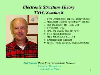
Electronic Structure Theory Session 7 Jack Simons, Henry Eyring Scientist and Professor Chemistry Department University of Utah
Multiconfigurational self-consistent field (MCSCF): the expectation value < | H | > / < | >, with = L CL1,L2,...LN |L1L2L...LN| is treated variationally and made stationary with respect to variations in both the CI and the C,icoefficients giving a matrix eigenvalue problem of dimension NC J HI,J CJ = E CI : with HI,J = < |I1I2I...IN|H| |J1J2J...JN|> and a set of HF-like equations for the C,I(but with more complicated Coulomb and exchange terms). Slater-Condon rules are used to evaluate the Hamiltonian matrix elements HI,Jbetween pairs of Slater determinants. IterativeSCF-like equations are solved to determine the CJ,coefficients of all the spin-orbitals appearing in any Slater determinant.
You must specify what determinants to include in the MCSCF wave function. Generally, one includes all determinants needed to form a proper spin- and spatial- symmetry correct configuration state function (CSF) or to allow for qualitatively correct bond dissociation: recall the1S function for carbon atom and the need for 2 and *2 determinants in olefins. This set of determinants form what is called a “reference space”. One then usually adds determinants that are doubly excited relative to any of the determinants in the reference space. The doubly excited determinants we know will be the most crucial for handling dynamical electron correlation. One can then add determinants that are singly, triply, etc. excited relative to those in the reference space. Given M orbitals and N electrons, there are of the order of N(M-N) singly excited, N2(M-N)2 doubly excited, etc. determinants. So, the number of determinants can quickly get out of hand.
The table below shows how many determinants can be formed when one distributes 2k electrons among 2k orbitals (4k spin-orbitals). Clearly, it is not feasible or wise to try to include in the MCSCF expansion all Slater determinants that can possibly be formed. Instead, one usually includes only determinants that are doubly or singly excited relative to any of the reference function’s determinants.
The HI,J matrix elements and the elements of the Fock-like matrix are expressed in terms of two-electron integrals < ij | e2/r1,2 | kl > that are more general than the Coulomb and exchange integrals. These integrals must be generated by “transforming” the AO-based integrals < ij | e2/r1,2 | kl > usingj = Cj,four times: < ij | e2/r1,2 | km> = l Cm,l < ij | e2/r1,2 | kl > < ij | e2/r1,2 | nmz> = k Cn,k < ij | e2/r1,2 | km> < ia | e2/r1,2 | nm > = j Ca,j < ij | e2/r1,2 | mm> < ba | e2/r1,2 | nm > = i Cb,i < ia | e2/r1,2 | mm> This integral transformation step requires of the order of 4 M5 steps and disk space to store the < ba | e2/r1,2 | nm >.
The solution of the matrix eigenvalue problem J HI,J CJ = E CI of dimension NC requires of the order of NC2 operations for each eigenvalue (i.e., state whose energy one wants). The solution of the Fock-like SCF equations of dimension M requires of the order of M3 operations because one needs to obtain most, if not all, orbitals and orbital energies. Advantages: MCSCF can adequately describe bond cleavage, can give compact description of, can be size extensive (give E(AB) = E(A) + E(B) when A and B are far apart) if CSF list is properly chosen, and gives upper bound to energy because it is variational. Disadvantages: coupled orbital (Ci,) and CIoptimization is a very large dimensional (iterative) optimization with many local minima, so convergence is often a problem; unless the CSF list is large, not much dynamical correlation is included.
Configuration interaction (CI): the LCAO-MO coefficients of all the spin-orbitals are determined first via a single-configuration SCF calculation or an MCSCF calculation using a small number of CSFs. The CIcoefficients are subsequently determined by making stationary the energy expectation value < | H | > / < | > which gives a matrix eigenvalue problem: J HI,J CJ = E CIof dimension NC. Advantages: Energies give upper bounds because they are variational, one can obtain excited states from the CI matrix eigenvalue problem. Disadvantages: Must choose “important” determinants, not size extensive, scaling grows rapidly as the level of “excitations” in CSFs increases (M5 for integral transformation; NC2per electronic state), NC must be larger than in MCSCF because the orbitals are optimized for the SCF (or small MCSCF) function not for the CI function.